Chapter Contents
Normalized Difference Vegetation Index (NDVI)
Remote sensing sensors record reflected or emitted energy. The reflected energy is recorded as reflectance, and the emitted energy is frequently converted to temperature. Onboard Landsat 8, the OLI and the TIRS sensors provide reflectance and temperature values, respectively.
Users, however, frequently need more than reflectance or temperature values. This chapter describes some popular datasets that are derived from the reflectance values.
Normalized Difference Vegetation Index (NDVI)
Vegetation indices are calculated from reflectance values. The most frequently used vegetation index is the normalized difference vegetation index (NDVI). NDVI is calculated as follows:
![]()
In the case of TM (Landsat 4 and 5) or ETM+ (Landsat 7) images, band 4 is the near-infrared band, and band 3 is the red band. Therefore, NDVI = (Band4 – Band3) / (Band4 + Band3). In the case of Landsat 8’s OLI, the near-infrared band and red bands are Band 5 and Band 4, respectively. Therefore, NDVI = (Band5 – Band4) / (Band5 + Band4).
When calculating NDVI from Landsat imagery using the above equation, problems may occur at abnormal pixels such as no-data and error pixels. Such pixels need to be filtered out during the NDVI calculation. In addition, some programs may return integer values if the red and near-infrared bands are recorded in integer values. Casting the integer values to float may resolve the potential integer output problem.
NDVI values range from -1.0 to +1.0, and NDVI is known to be directly related to the photosynthesis of vegetation. Typically, vegetation has high NDVI values. NDVI has been used for various vegetation applications such as urban canopy, forest monitoring, and crop monitoring. Global land cover change analysis and crop type identification have also been performed using multiple NDVI images in time series.
Figure 1 shows an NDVI image in Atlanta and vicinity on May 6, 2020.
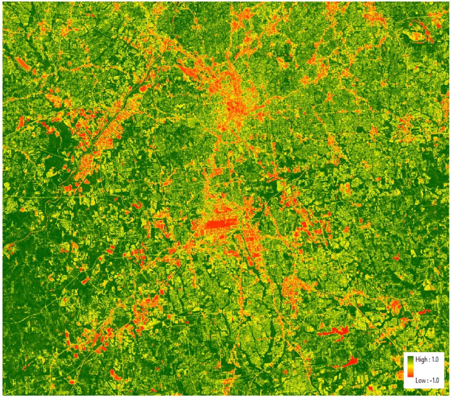
Figure 1. NDVI values calculated from Landsat 8 ARD dataset. Atlanta and vicinity. 2020-05-06.
Tasseled-Cap Transformation
The Tasseled-cap transformation is a linear conversion method using equations such as [Output = a x B1 + b x B2 …], where B indicates band, and the parameters a, b, … are calculated from empirical experiments. Brightness, greenness, and wetness are typically calculated as the output. The term “Tasseled-cap” is from the shape of a scatter plot with near-infrared and red bands. As shown in Figure 2, their scatterplot is like a tasseled-cap. In the image, the green color indicates high frequency, and the blue color indicates low frequency. The red polygon was draped on the scatterplot to symbolize a tasseled-cap shape.
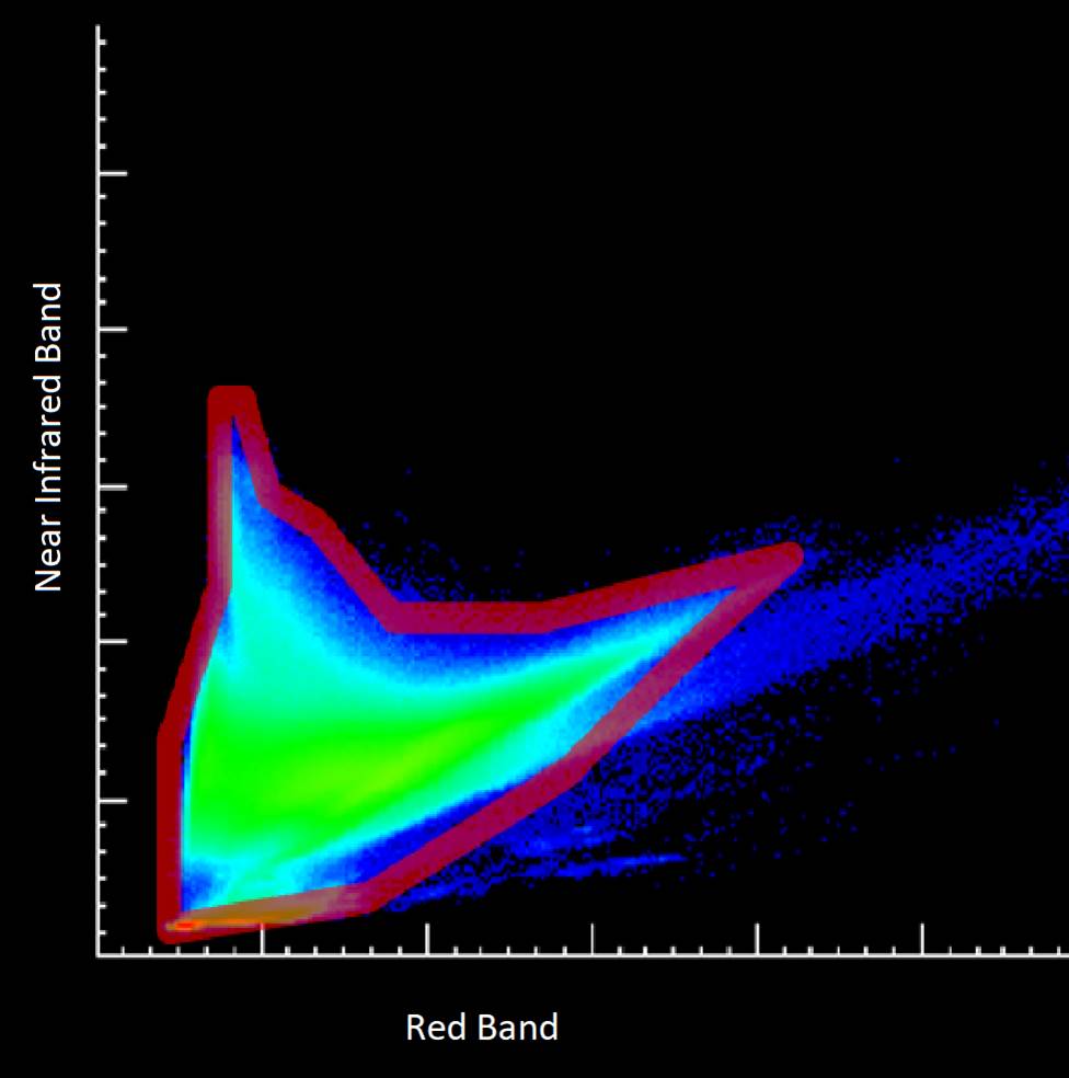
Figure 2. A scatterplot of a red band and a near-infrared band of a Landsat 5 TM image.
The tasseled-cap transformation has been used since the Landsat MSS sensor was used. The following tables show the tasseled-cap parameters for Landsat MSS, TM, ETM+, and OLI sensor images.
Table 1. The tasseled-cap parameters for Landsat MSS sensor. (Kauth and Thomas, 1976).
|
Output |
Band 1 |
Band 2 |
Band 3 |
Band 4 |
|
Brightness |
0.433 |
0.632 |
0.586 |
0.264 |
|
Greenness |
-0.290 |
-0.562 |
0.600 |
0.491 |
|
Yellowness |
-0.829 |
0.522 |
-0.039 |
0.194 |
|
"Non-such" |
0.223 |
0.012 |
-0.543 |
0.810 |
Table 2. The tasseled-cap parameters for Landsat TM sensor. (Crist and Cicone, 1984)
|
Output |
Band 1 |
Band 2 |
Band 3 |
Band 4 |
Band 5 |
Band 7 |
|
Brightness |
0.3037 |
0.2793 |
0.4743 |
0.5585 |
0.5082 |
0.1863 |
|
Greenness |
-0.2848 |
-0.2435 |
-0.5436 |
0.7243 |
0.0840 |
-0.1800 |
|
Wetness |
0.1509 |
0.1973 |
0.3279 |
0.3406 |
-0.7112 |
-0.4572 |
Table 3. The tasseled-cap parameters for Landsat ETM+ sensor. (Hwang, et al., 2002)
|
Output |
Band 1 |
Band 2 |
Band 3 |
Band 4 |
Band 5 |
Band 7 |
|
Brightness |
0.3561 |
0.3972 |
0.3904 |
0.6966 |
0.2286 |
0.1596 |
|
Greenness |
-0.3344 |
-0.3544 |
-0.4556 |
0.6966 |
-0.0242 |
-0.2630 |
|
Wetness |
0.2626 |
0.2141 |
0.0926 |
0.0656 |
-0.7629 |
-0.5388 |
|
Fourth |
0.0805 |
-0.0498 |
0.1950 |
-0.1327 |
0.5752 |
-0.7775 |
|
Fifth |
-0.7252 |
-0.0202 |
0.6683 |
0.0631 |
-0.1494 |
-0.0274 |
|
Sixth |
0.4000 |
-0.8172 |
0.3832 |
0.0602 |
-0.1095 |
0.0985 |
Table 4. The tasseled-cap parameters for Landsat OLI sensor. (Baig, et al., 2014)
|
Output |
Band 2 |
Band 3 |
Band 4 |
Band 5 |
Band 6 |
Band 7 |
|
Brightness |
0.3029 |
0.2786 |
0.4733 |
0.5599 |
0.5080 |
0.1872 |
|
Greenness |
-0.2941 |
-0.2430 |
-0.5424 |
0.7276 |
0.0713 |
-0.1608 |
|
Wetness |
0.1511 |
0.1973 |
0.3283 |
0.3407 |
-0.7117 |
-0.4559 |
|
Fourth |
-0.8239 |
0.0849 |
0.4396 |
-0.0580 |
0.2013 |
-0.2773 |
|
Fifth |
-0.3294 |
0.0557 |
0.1056 |
0.1855 |
-0.4349 |
0.8085 |
|
Sixth |
0.1079 |
-0.9023 |
0.4119 |
0.0575 |
-0.0259 |
0.0252 |
In calculating the tasseled-cap outputs with the above parameters, the at-satellite reflectance values are used.
Example
The following image shows the reflectance values at a point in a Landsat 8 OLI ARD dataset. With the reflectance values of the pixel (“x”) in the figure, tasseled-cap outputs are calculated as follows:
· Brightness = 0.3029 * 0.1029 + 0.2786 * 0.1002 + 0.4733 * 0.0850 + 0.5599 * 0.3303 + 0.5080 * 0.2378 + 0.1872 * 0.1238
· Greenness = -0.2941 *0.1029 - 0.2430 * 0.1002 - 0.5424 * 0.0850 + 0.7276 * 0.3303 + 0.0713 * 0.2378 - 0.1608 * 0.1238
· Wetness = 0.1511 * 0.1029 + 0.1973 * 0.1002 + 0.3283 * 0.0850 + 0.3407 * 0.3303 - 0.7117 * 0.2378 - 0.4559 * 0.1238
And calculating them gives:
· Brightness = 0.428
· Greenness = 0.137
· Wetness = -0.050
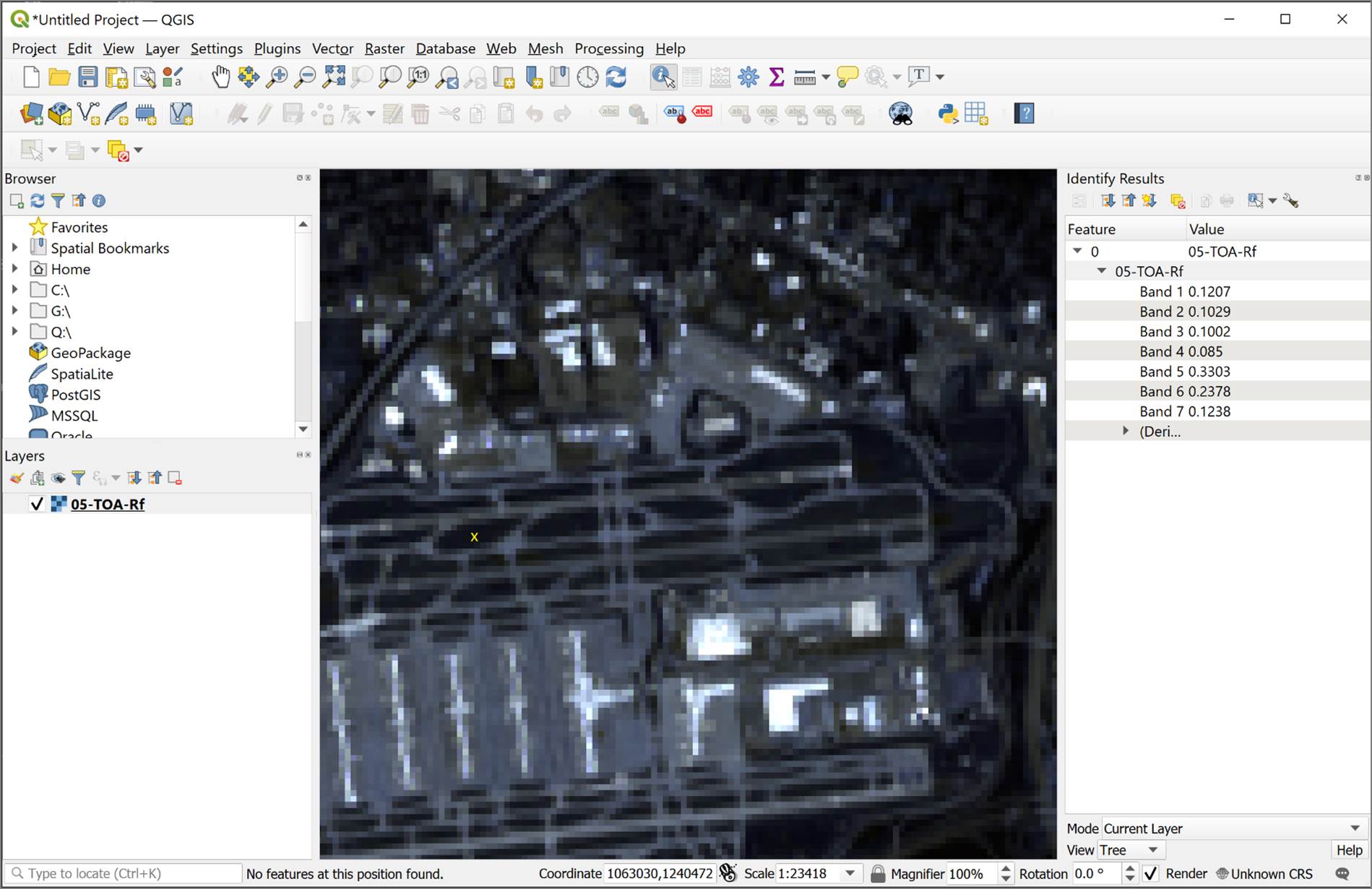
Figure 3. The at-satellite reflectance values for the pixel (“x”) on a grass patch between runways. Atlanta Hartsfield International Airport. Landsat 8 OLI image. May 6, 2020.
Principal Components
Principal components transformation, also known as principal components analysis, changes multiple bands to multiple principal components. Typically, the first couple of components carry most of the original information. Principal components transformation is good for reducing data volumes while keeping most of the original information.
Figure 4 shows very high correlations among bands. As shown in the table, Pearson’s correlation coefficients between bands are higher than 0.89, indicating significant information redundancy among bands.
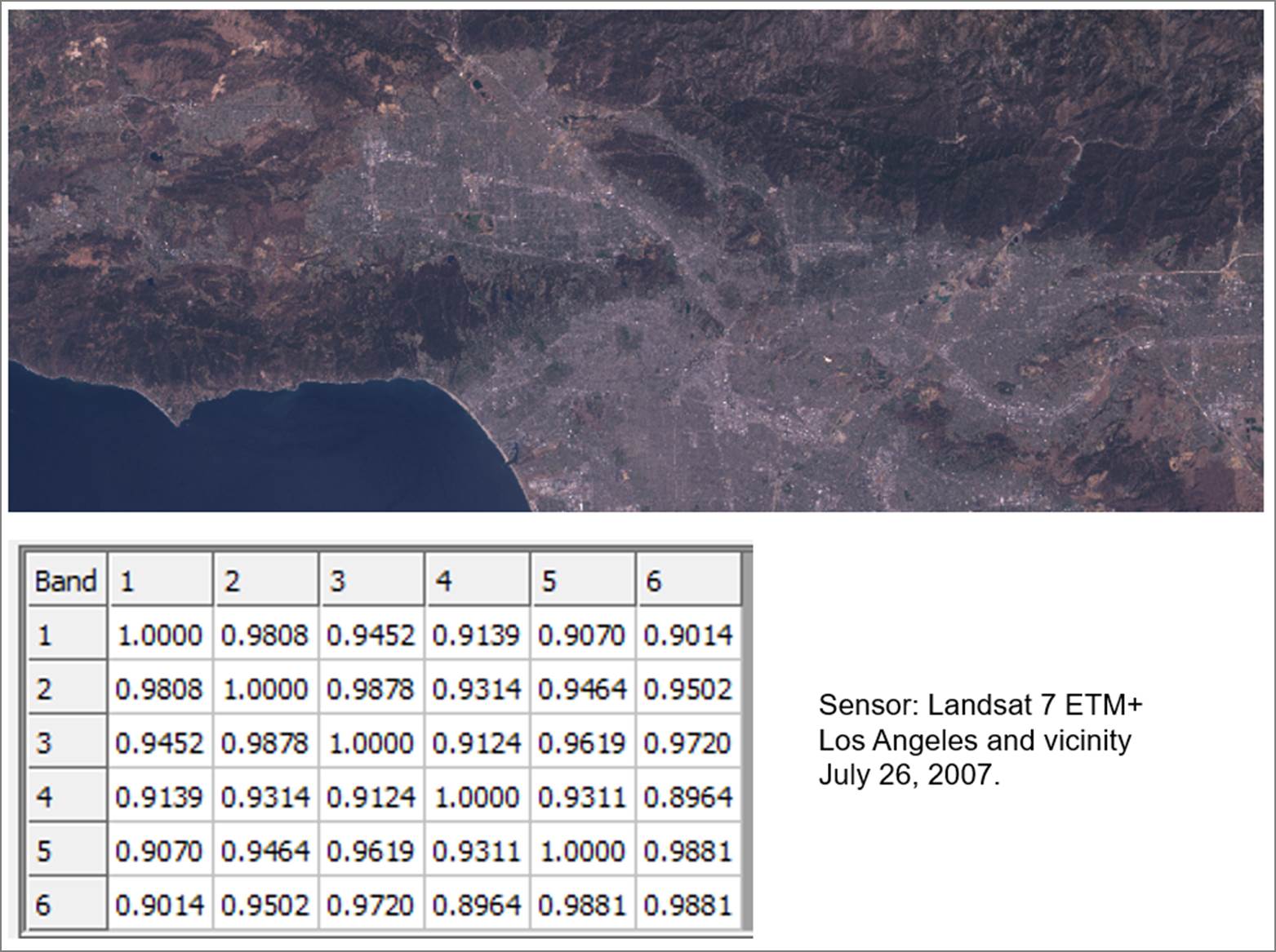
Figure 4. Correlation among bands. Band number 6 in the figure indicates the Band 7.
Figure 5 shows the result of principal components transformation. As shown in the figure, the first principal component explains 96.04% of original information, and the second explains 2.31%. It also shows the association between principal components and original bands. For example, principal component #1 (i.e. PC1) is highly correlated with all six bands; and PC3 with Band 4.
Using the principal components as they are is very challenging because it is difficult to find the meaning of each principal component. Rather, the principal components transformation has been used for further analyses so that computational workloads can be reduced significantly. Particularly, processing hyperspectral or multitemporal images that often have hundreds of bands or layers might benefit from the principal component transformation.
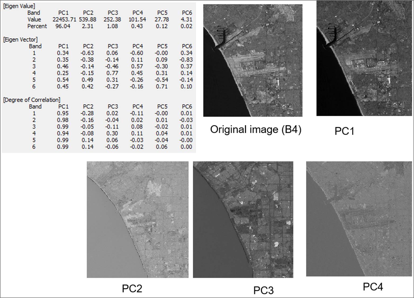
Figure 5. Principal components derived from an ETM+ image. Los Angeles and vicinity. July 26, 2007.
Application Example
With global climate change, understanding the relationship between land surface temperature (LST) and NDVI or tasseled-cap transformation may help practitioners or decision makers to understand their communities. The OLI and TIRS sensors onboard Landsat 8 provide an opportunity to analyze the relationship between physical parameters and LST.
Figure 6 shows a Landsat image with sampling sites, and the derived datasets of LST, brightness, greenness, and wetness. Figure 7 shows their relationships measured at the sample points. The figure shows that LST is positively correlated with brightness, but negatively correlated with greenness, NDVI, and wetness. This simple analysis may support various environmental initiatives such as planting more trees to reduce regional land surface temperature.
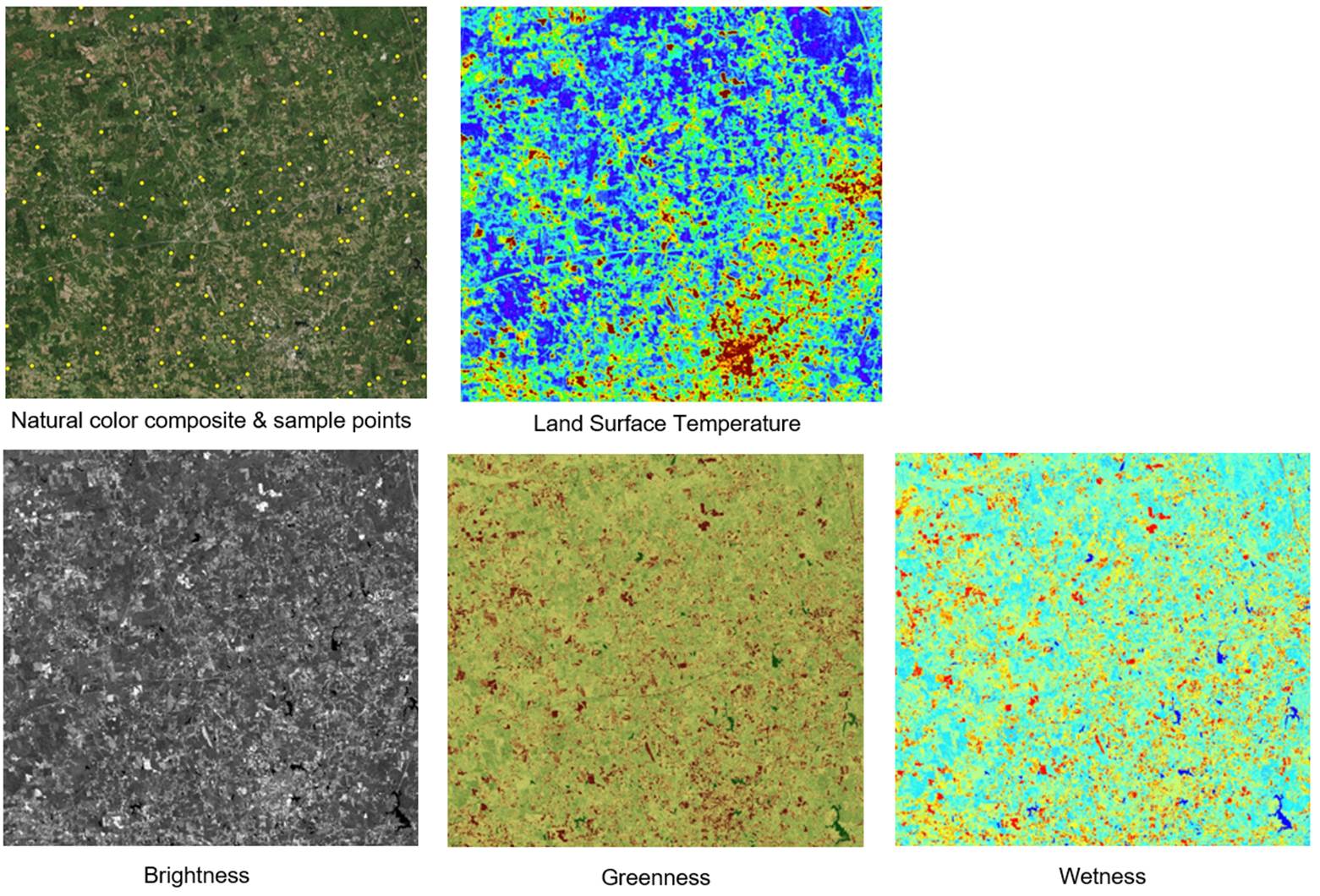
Figure 6. Land surface temperature and tasseled-cap transformations. Landsat 8. Carrollton, GA, and vicinity. The image was taken on May 14, 2017.
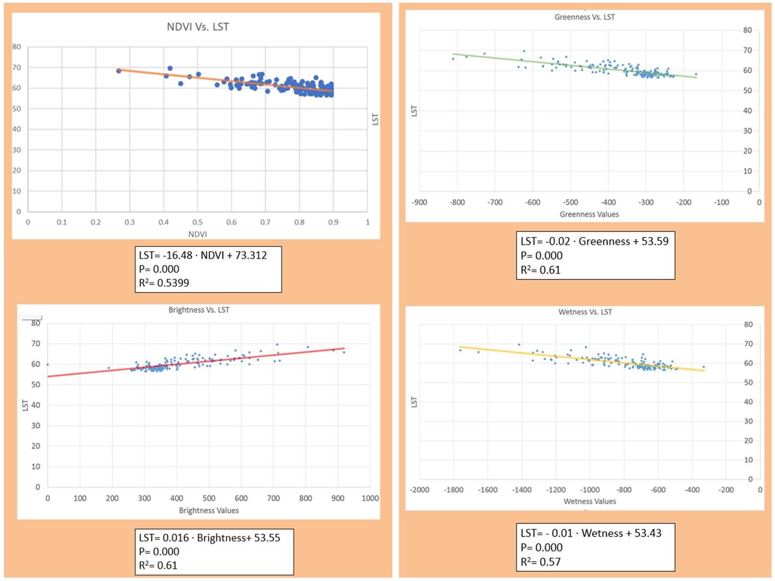
Figure 7. The relationships between LST and NDVI, greenness, brightness, and wetness.
References
Kauth, R.J. and Thomas, G.S., 1976. The Tasselled Cap—A Graphic Description of the Spectral-Temporal Development of Agricultural Crops as Seen by LANDSAT. LARS Symposia, paper 159.
Crist, E.P. and Cicone, R.C., 1984. A physically based transformation of Thematic Mapper data—The TM Tasseled Cap, IEEE Transactions on Geosciences and Remote Sensing, GE-22: 256–263.
C. Huang,B. Wylie,L. Yang,C. Homer and G. Zylstra, 2002. Derivation of a tasseled cap transformation based on Landsat 7 at-satellite reflectance. International Journal of Remote Sensing 23: 1741–1748.
Muhammad Hasan Ali Baig, Lifu Zhang, Tong Shuai and Qingxi Tong, 2014. Derivation of a tasselled cap transformation based on Landsat 8 at-satellite reflectance, Remote Sensing Letters, 5:5, 423-431, DOI: 10.1080/2150704X.2014.915434