Chapter Contents
This chapter introduces some techniques for enhancing images for visual analyses. Particularly, contrast enhancement, pan-sharpening, and spatial filtering are introduced.
Contrast Enhancement
The contrast of a digital image can be changed dramatically depending on how the pixel values are represented on a screen. Most raw images have low contrast as shown in Figure 1.
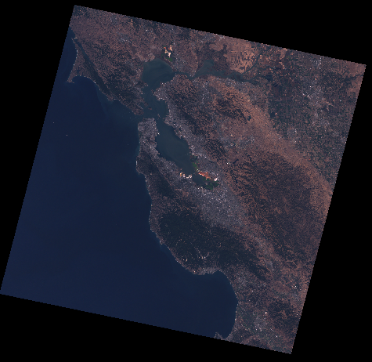
Figure 1. An example of a raw image without any contrast enhancement. Landsat 7 ETM+ image. San Francisco and vicinity. September 30, 2001.
Multiple contrast enhancement algorithms and techniques have been developed. Some popular algorithms are min-max linear stretch, histogram equalization, logarithmic, inverse square root, and standard deviation.
Min-Max Linear Stretch
The min-max linear stretch method stretches pixel values linearly. For example, suppose stretching [3, 5, 6, 7, and 9] to the 0-255 range.
· 3 is the minimum so it will be changed to 0.
· 9 is the maximum so it will be stretched to 255.
· 5, 6, and 7 will be stretched proportionally using the following equation:
![]()
(ex.) The value 5 will be stretched to 85 = (5 – 3) / (9 – 3) x 255.
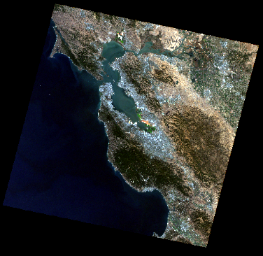
Figure 2. Result of a min-max linear stretch
Histogram Equalization
Histogram equalization method flattens a histogram using probabilities. It uses multiple steps to flatten a histogram as shown in Figure 3. First, the ratio, probability, and cumulative probability are calculated for each pixel (=DN) value. Second, the nearest ratio is searched for each cumulative probability. Finally, the nearest ratios are stretched to a 0 – 255 scale. Figure 4 shows the result of histogram equalization.
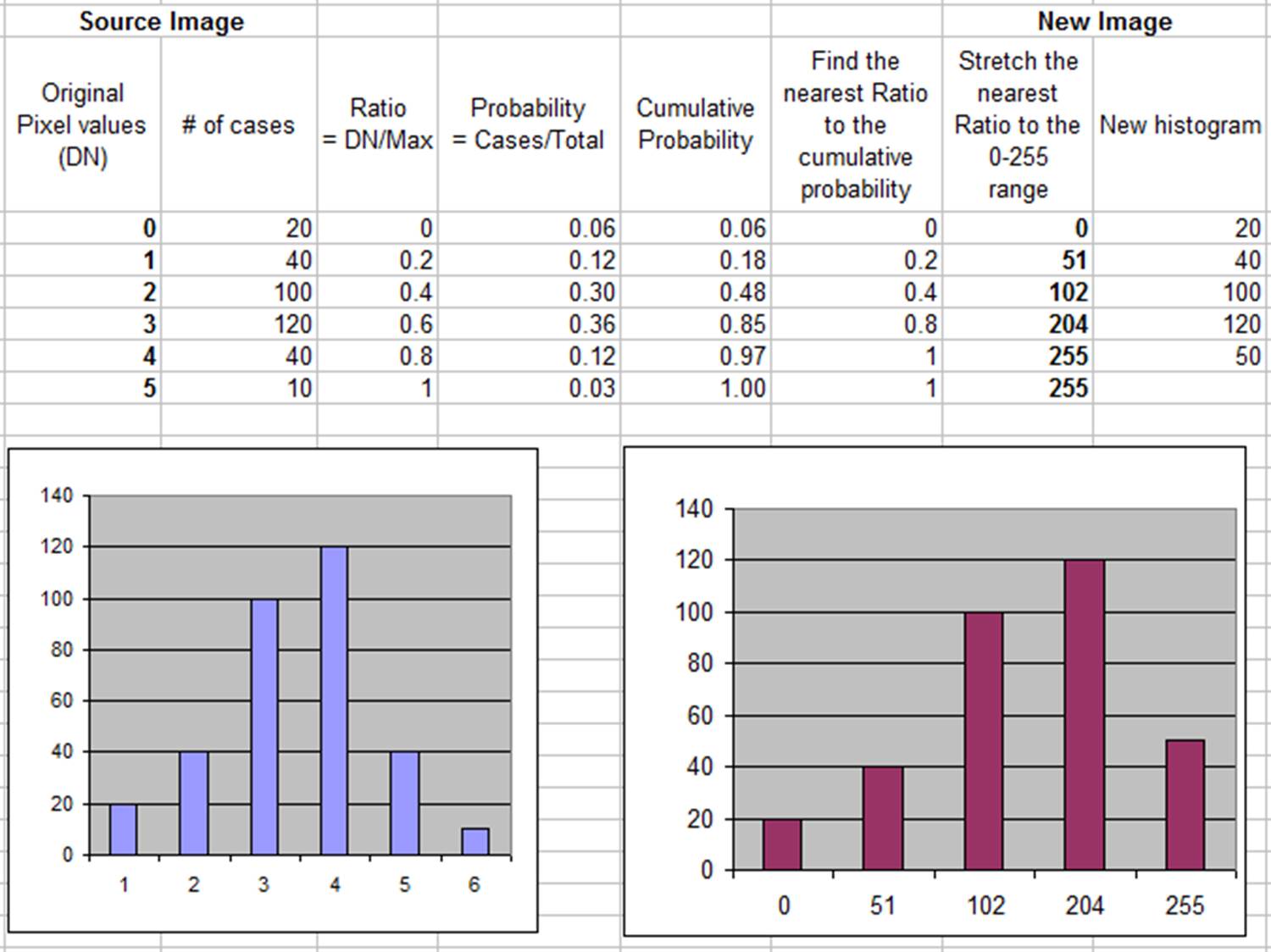
Figure 3. Histogram equalization procedure.
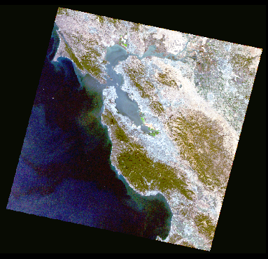
Figure 4. Result of histogram equalization
Logarithmic Stretch
The logarithmic stretch uses a log function. Darker tones are stretched more than the light tones as shown in Figure 5. In the figure, the x-axes indicate pixel values, and the y-axes indicate frequencies. Histograms appear along the x-axes. The yellow-tinted parts show a dramatic stretch in the smaller pixel value range. Figure 6 shows the result of logarithmic stretch. Subtle differences are well represented in the originally dark tone features such as water.
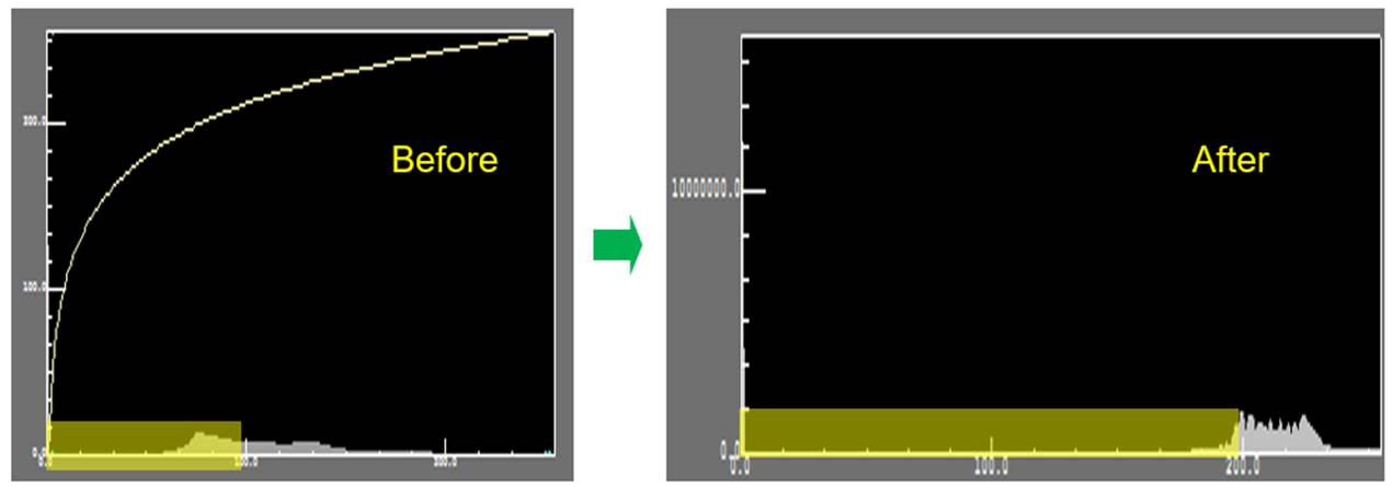
Figure 5. Logarithmic stretch mechanism.
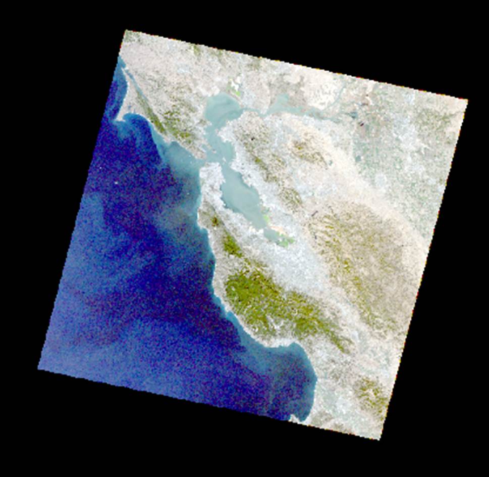
Figure 6. Result of logarithmic stretch
Inverse Square Root Stretch
The Inverse square root method enhances more the details of the brighter pixels. Darker pixels are suppressed further. Figure 7 shows how the inverse square root stretch works. As shown in Figure 8, the originally brighter pixels like urban areas and open lands are enhanced with further details, but the originally darker pixels like water are further suppressed.
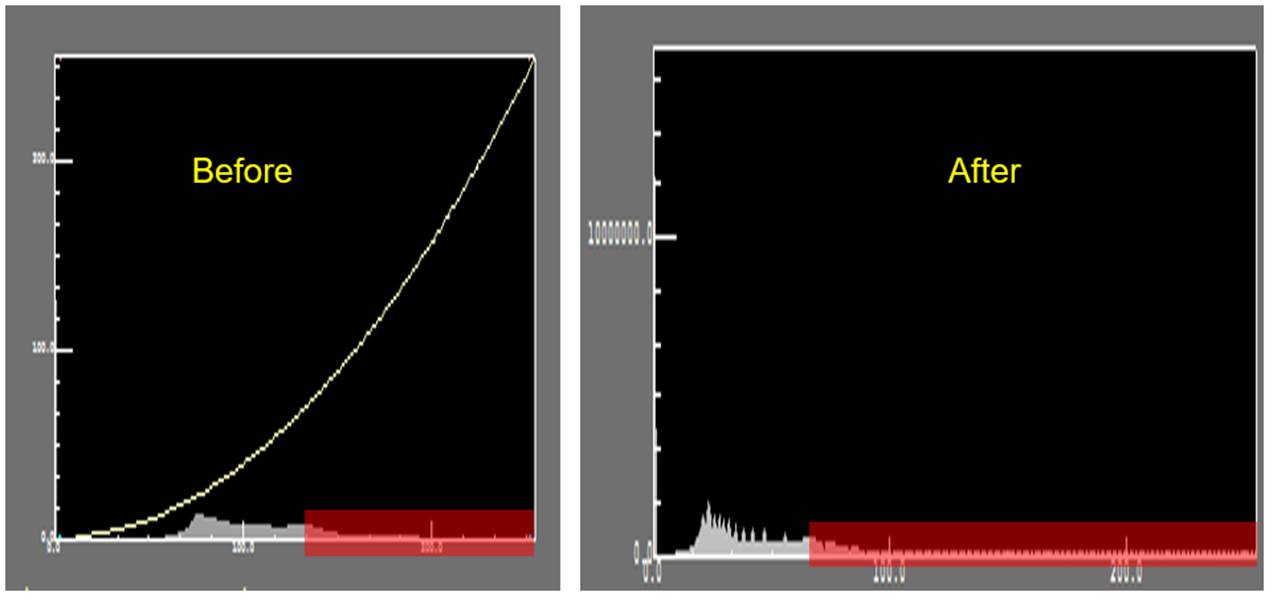
Figure 7. Inverse square root stretch mechanism.

Figure 8. Result of inverse square root stretch.
Standard Deviation Stretch
The standard deviation method stretches the pixel values that are within a pre-defined standard deviation distance from the mean of pixel values in each band. Because the standard deviation method used the mean value in each band, it stretches mid-tone pixels very well. In the standard deviation stretch, the pixel values outside of the standard deviation distance are not stretched, but rather suppressed. Figure 9 shows that the mid-tones like vegetation are well represented.
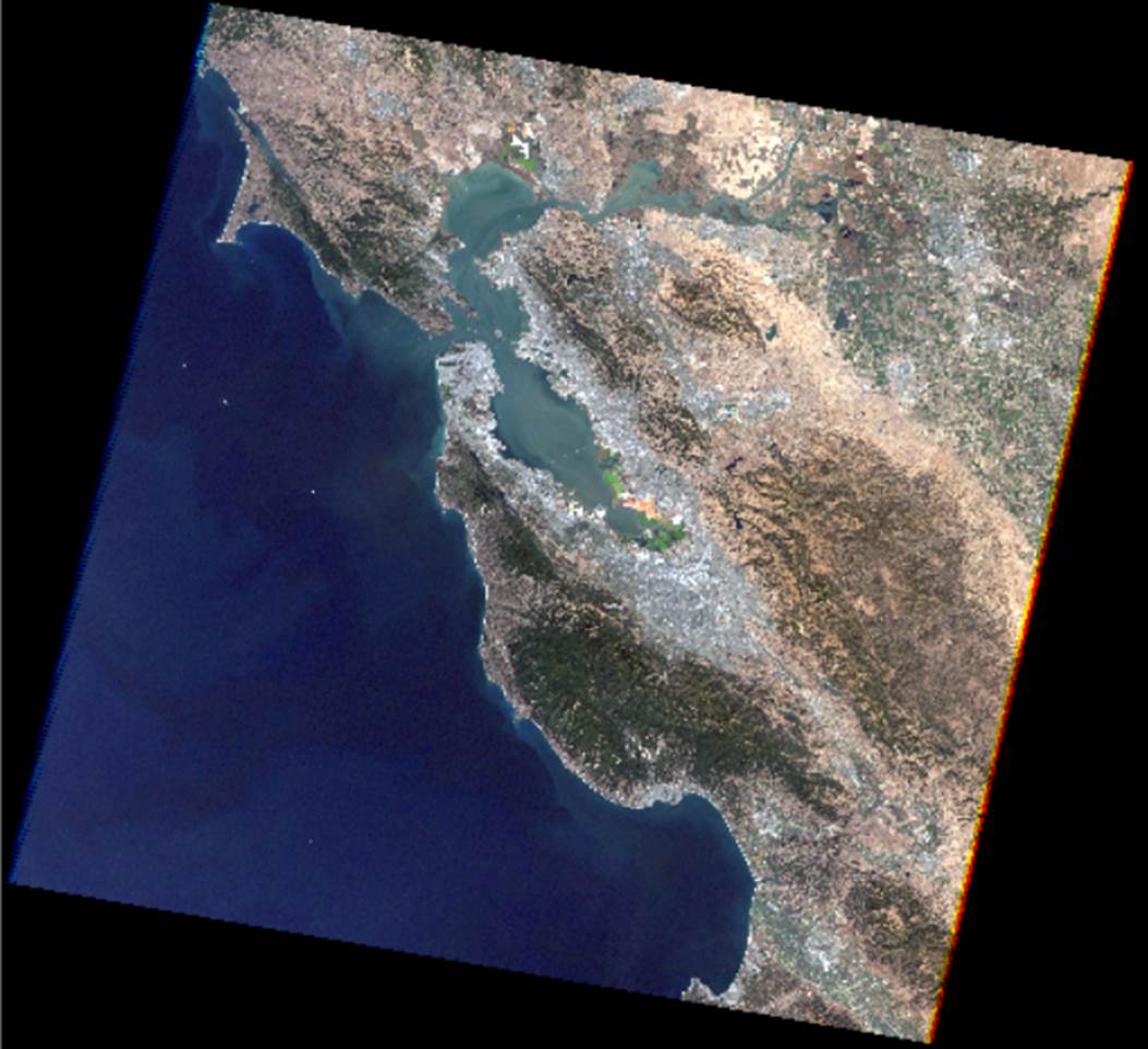
Figure 9. Result of standard deviation stretch. (Standard deviation = 2.5)
Pan-Sharpening
Pan sharpening is used to increase the spatial resolution of multispectral (color) image data by using a higher-resolution panchromatic image. Most Earth resource satellites such as SPOT and Landsat provide multispectral images at a lower spatial resolution and a panchromatic image at a higher spatial resolution. In the case of Landsat 8 OLI, Band 8 is the panchromatic band and its spatial resolution is 15 m, while other bands’ spatial resolution is 30 m.
It is also possible to use different sensor image to perform pan sharpening. Two pan-sharpening methods are used frequently - IHS transformation and Brovey transformation.
HIS Transformation
Figure 10 shows the HIS transformation procedure. In the IHS transformation, original RGB bands are transformed to IHS (intensity, hue, and saturation) using the equation shown at the lower left corner. Then, the intensity band is replaced with a higher resolution gray-scale image, Layer I’. The bright green color layer in the diagram is a higher resolution image. Finally, I’HS layers are converted back to RGB layers to make a pan-sharpened image. In this procedure, the histograms of Layer I’ is usually adjusted to be matched to Layer I.
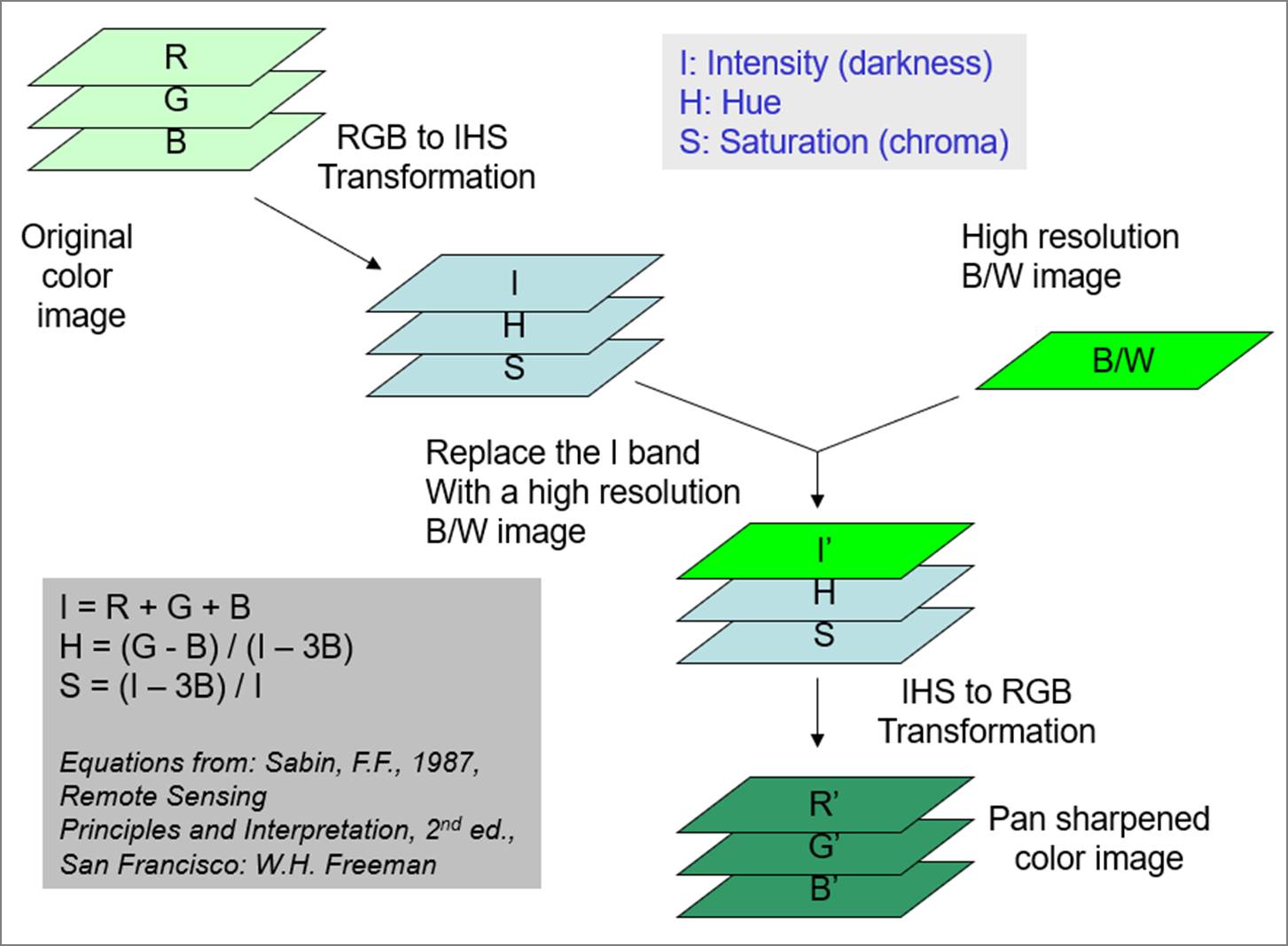
Figure 10. Pan-sharpening using the IHS transformation method.
Brovey Transformation
Brovey transformation is simpler than the HIS transformation. Brovey transformation visually increases the contrast in the low and high ends of an image’s histogram. In the Brovey transformation, the intensity is calculated with RGB bands. Then, new RGB layers are calculated with a higher resolution panchromatic layer and the intensity layer. Equations are shown below.
I = (Red + Green + Blue) / 3
P: Higher resolution band (ex. panchromatic band)
Rednew = (Red x P) / I
GreenNew = (Green x P) / I
BlueNew = (Blue x P) / I
Example
Figure 11 shows an example of pan-sharpening with a Landsat 7 ETM+ image. The panchromatic band has a higher spatial resolution, i.e. 15m compared with 30m, but it lacks in color. On the contrary, the multispectral composite image has color but carries lower spatial resolution, i.e. 30m. The result of a pan-sharpening with the HIS transformation in the figure shows an improved spatial resolution with colors.
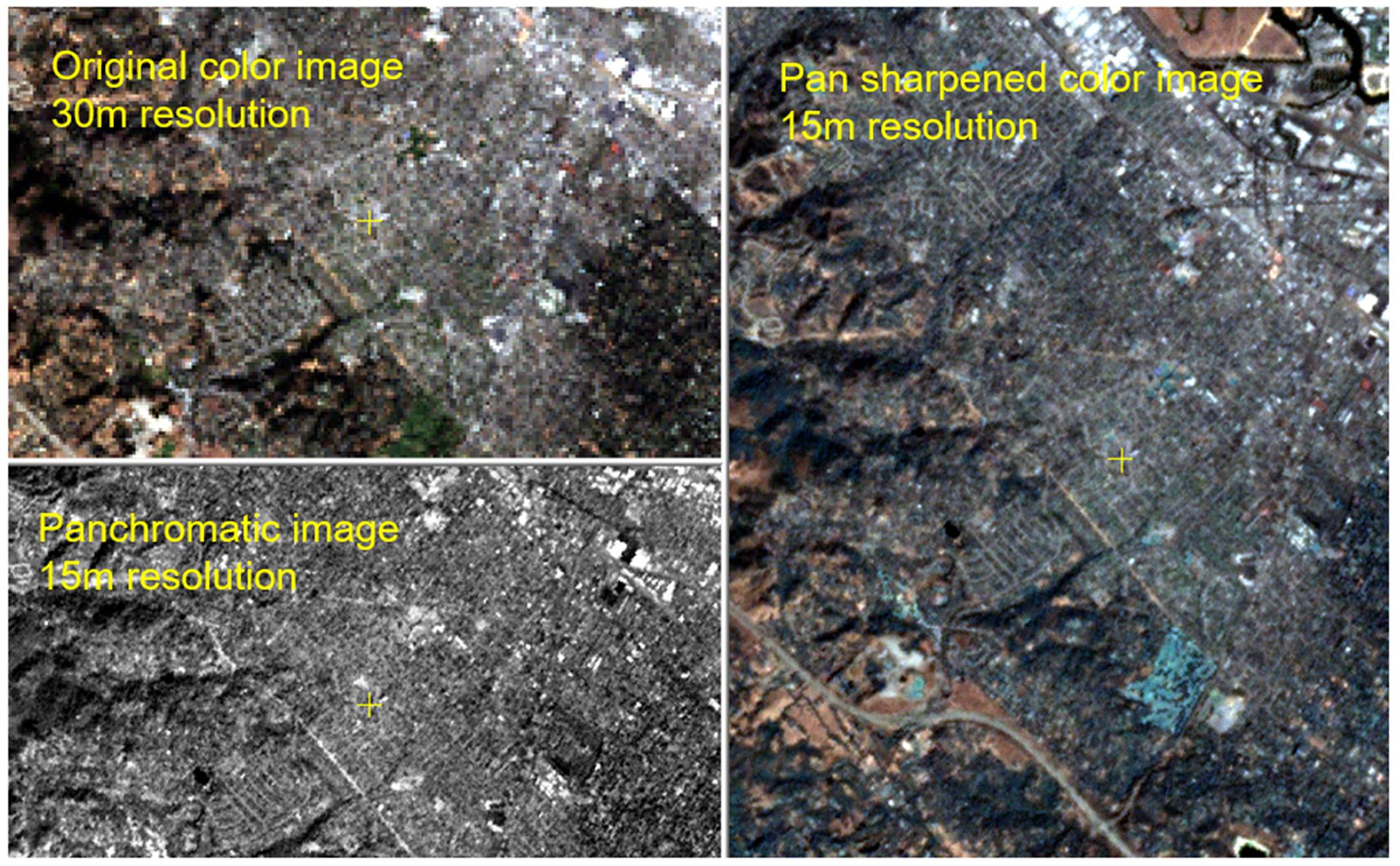
Figure 11. Result of pan-sharpening. Landsat ETM+. San Francisco area. September 30, 2001.
Spatial Filtering
An image can be characterized by various frequencies. Low frequencies carry smoothly changing information such as forest and water. High frequencies carry abruptly changing information such as urban areas. Spatial filters can be applied to filter specific frequencies depending on applications. Two filtering approaches are often used. One is to use convolution filters, and the other is to use the Fourier Transformation.
Convolution Filters
A convolution filter is a 2-D moving window in which pixels contain weighting values. For example, A 3 X 3 mean filter contains a weighting value of 1.0 in each pixel, and the new value of the center pixel is the mean of all nine values.
DN2,2_New = ( 1.0 x DN1,1 + 1.0 x DN1,2 + 1.0 x DN1,3
+ 1.0 x DN2,1 + 1.0 x DN2,2 + 1.0 x DN2,3
+ 1.0 x DN3,1 + 1.0 x DN3,2 + 1.0 x DN3,3
) / 9.0
In a generalized form, the new DN value at the center of the filter is the sum of the weighting value multiplied by pixel value, divided by the total number of pixels in the moving window.
DNNew = ∑(W x V) / n
Where, W: weighting value
V: DN value
n: total number of pixels in the filter
Even though a 3x3 moving window is most popular, many other shapes of moving window are possible, such as 5x5, 7x7, and octagonal array shape as shown in Figure 12.
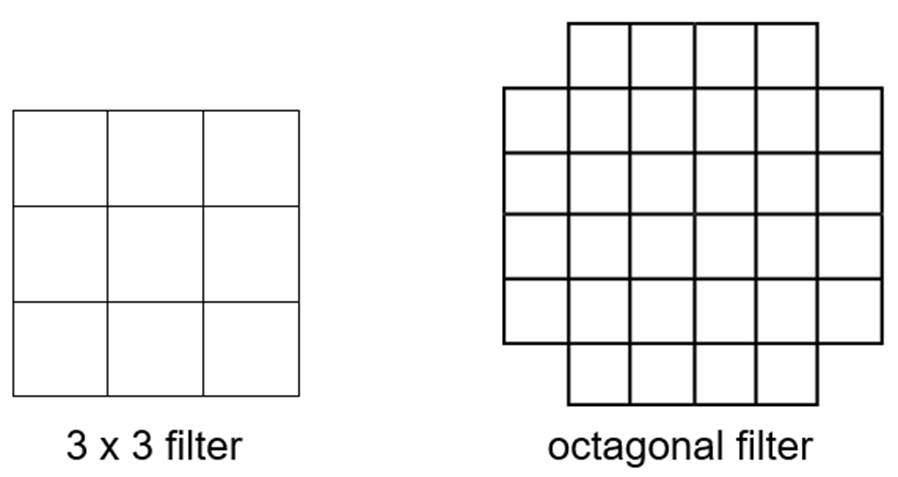
Figure 12. Examples of convolution filters.
There are many weighting methods, and they can be grouped into two categories --low pass filters and high pass filters.
Low pass filters allow low-frequency signals to pass through, resulting in smoothly changing tones appearing in the output image. One example is a 3x3 mean filter as shown in Figure 13. The output image becomes blurry. Low pass filters are frequently used to remove abnormal noises in an image.
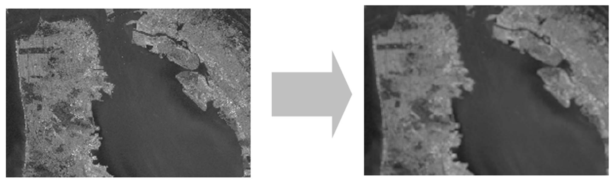
Figure 13. Result of applying the 3x3 mean filter.
High pass filters allow high frequencies (or sharply changing signals) to appear in the output image. Smoothly changing low frequencies are filtered out. One example is the edge enhancement filter with the weighting values as shown below.
3x3 edge enhancement filter (ex).
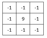
Figure 14 shows the result of applying the edge enhancement filter.

Figure 14. Result of applying the 3x3 edge enhancement filter.
Fourier Transformation
Fourier transformation is another popular technique for editing frequencies. With the Fourier transformation, an image is changed from the spatial domain to the frequency domain, or vice versa. Once an image is converted to the frequency domain, certain frequency information can be removed or modified.
Figures 15 shows what low and high frequencies are. Figures 16 and 17 show examples of applying the Fourier transformation technique. In Figure 16, for example, the original image is in the spatial domain. After Fourier transformation, the lower left image is acquired that is in the frequency domain. After modifying the frequency domain (e.g. trimming the frequencies larger than 2047 in this example), inverse Fourier transformation equations are applied to transform an image from the frequency domain to the spatial domain. The right-hand side image shows the result of applying inverse Fourier transformation equations, which is the final outcome.
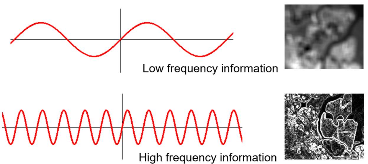
Figure 15. Low and high frequency information in an image
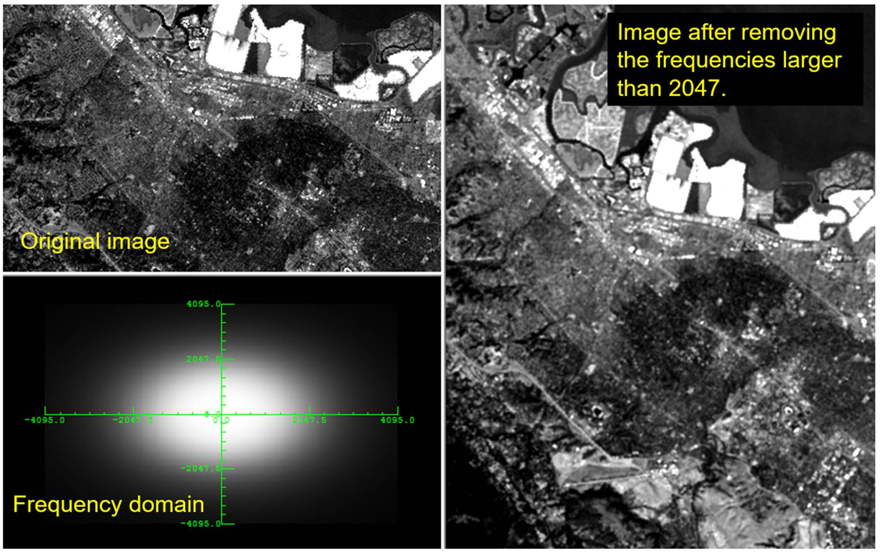
Figure 16. Fourier transformation to remove the frequencies larger than 2047. Note: In the frequency domain of this example, the frequency values in the x and y axes do not represent real frequencies. Real frequencies were scaled down to the [-4095 - 4095] range.
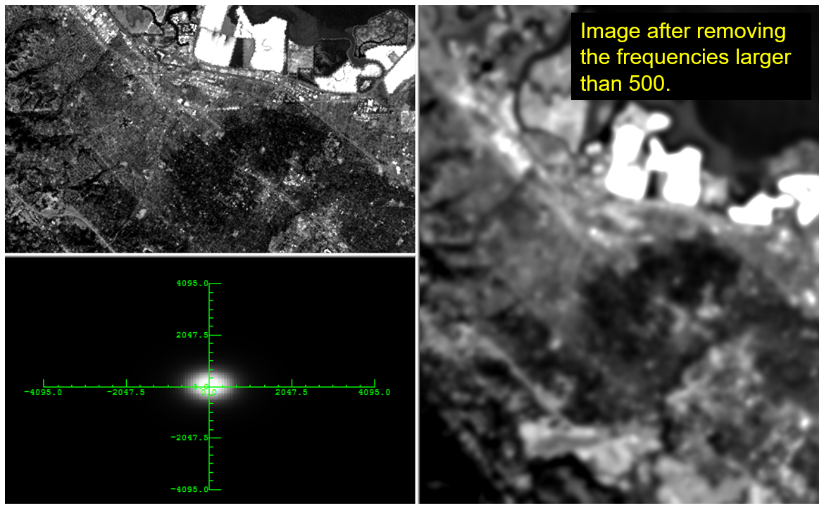
Figure 17. Fourier transformation to remove the frequencies larger than 500.