Chapter Contents
Sensor Geometry and Scene Referencing
MODIS Instrument Onboard Terra and Aqua Satellites
Satellites, airplanes, drones, balloons, and kites are popular vehicles that carry remote sensing sensors. This chapter will focus on earth imaging satellites and the sensors onboard them.
Satellite Characteristics
There are thousands of artificial satellites in the space. Most of them are used for imaging the Earth, and for communication and broadcasting. Commercial satellites (e.g. WorldView-3) often provide high resolution (i.e. small pixel size) images, while weather and scientific satellites (e.g. Landsat, Terra, and GOES) provide mid- and coarse-resolution images.
Orbit Period
Understanding how satellites orbits a planet helps us to figure out when images are taken. The orbit period means the time to make one orbit. A satellite’s orbit period is directly related to the satellite’s altitude, and it is calculated with the equation shown below. In the equation, R is the planet radius (about 6380km for the Earth), H is the orbital altitude above the Earth’s surface, and g is the gravitational acceleration at the Earth’s surface (i.e. 0.00981km/sec2 for the Earth).
For example, if a satellite orbits 400km above the Earth’s surface, its orbit period can be calculated with the following equation in Excel, and the orbit period will be about 1.54 hours.
= 2 * 3.14159 * (6380 + 400) * SQRT( (6380 + 400) / (0.00981 * 6380^2) )
= 5551 seconds, which is 1.54 hours.
From the equation, we can also calculate the altitude for a specific orbit period. As an example, an altitude of 36,000km is needed to have a 24-hour orbit period.
One thing interesting is that an increase of a satellite’s speed with its thrusters does not increase the orbit period. Suppose a satellite operator fires the thrusters to accelerate the satellite. Then, it will boost the orbit and increase the altitude, which will eventually slow the orbital speed and increase its orbit period. Instead, firing the thrusters in a direction opposite to the satellite’s forward motion will push the satellite into a lower orbit, which will increase its forward velocity and decrease its orbit period.
Three Major Satellite Altitudes
Satellites altitudes can be grouped into three zones:
· Low altitude zone: 180 - 2,000 km
· Mid altitude zone: 2,000 – 35,780 km
· High altitude zone: 35,780 -
High and mid resolution earth imaging satellites are mostly placed at the low altitude zone. For example, the Landsat-8 satellite’s altitude is about 705 km. Global navigation satellites like GPS satellites are mostly placed in the mid-altitude zone. In the case of GPS satellites, their altitude is about 20,200 km with an orbit period of about 12 hours. Weather and communication satellites are mostly placed in the high altitude zone. Particularly, the altitude of about 36,000 is very popular because its orbit period is about 24 hours.
Geostationary Satellites
If a satellite orbits the Earth with the orbit period of 24 hours on the equatorial plane, the people on the Earth will perceive the satellite to be stationary because the Earth’s revolution is also about 24 hours. This kind of satellite is called a geostationary satellite. As mentioned in the previous section, the altitude of 36,000km provides about a 24-hour orbit period. Geosynchronous is another term for geostationary. Because geostationary satellites cover the same region all the time, they are used for communications and weather monitoring. Figures 1 and 2 show the location of geostationary satellites and a GOES-13 image as an example.
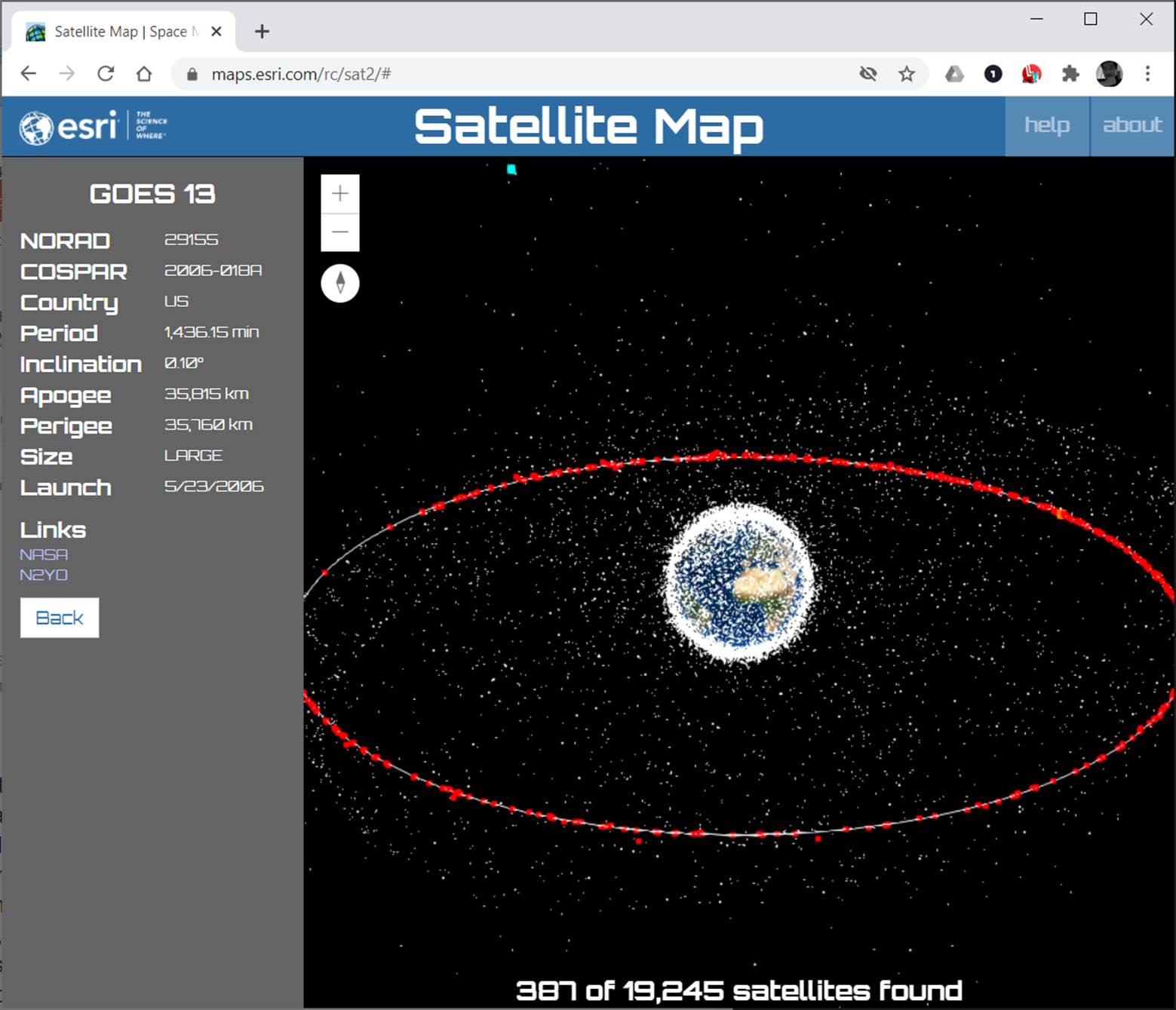
Figure 1. Geostationary satellites and the GOES-13 weather satellite. (URL: https://maps.esri.com/rc/sat2)
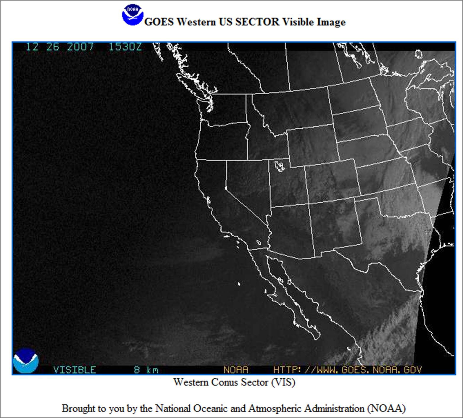
Figure 2. A weather image taken from the GOES satellite.
Inclination and Polar Orbiters
The Earth-observing satellites in the low altitude zone are frequently designed to pass the equator close to the right angle. The angle made by the equator and a satellite’s orbital path is the inclination. Because the inclination angle of about 90 degrees makes satellites pass the polar area, those satellites are called near-polar orbiters. Figure 3 shows the 98.22 degree inclination of Landsat-8.
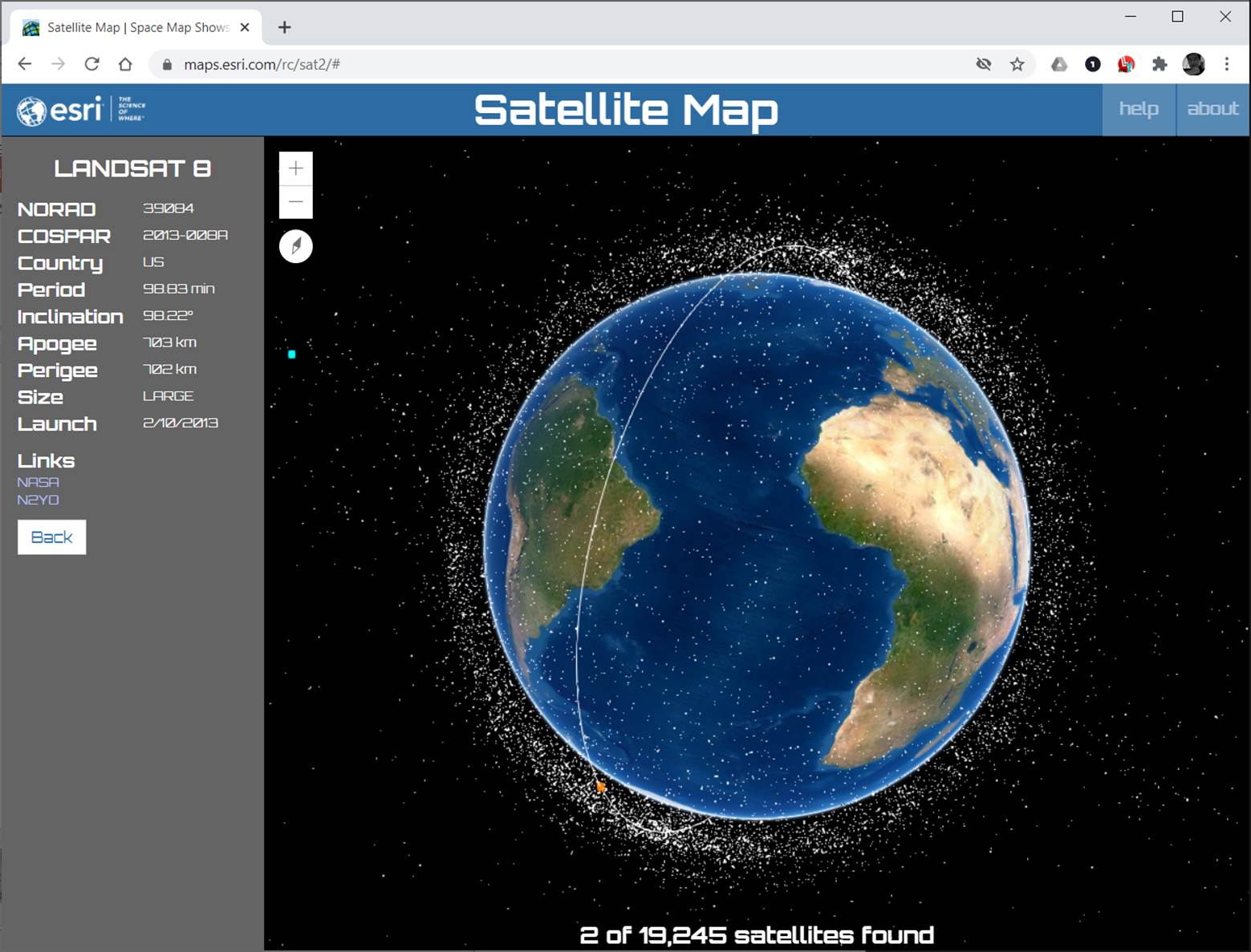
Figure 3. The inclination of Landsat-8’s orbit.
With the near polar orbits, there are ascending and descending paths as shown in Figure 4. The ascending path is the northward path, and the descending path is southward. Many of polar orbits are sun-synchronous such that they cover each area of the world at a constant local time of day called local sun time. At any given latitude, the position of the sun in the sky as the satellite passes overhead will be the same within the same season. This ensures consistent illumination conditions when acquiring images in a specific season over successive years or a particular area over a series of days.
If an orbit is sun-synchronous, the ascending pass is most likely on the shadowed side of the Earth while the descending pass is on the sunlit side. The sensors that record the reflected solar energy only image the Earth’s surface during the descending pass, when solar illumination is available. Active sensors that provide their own illumination or passive sensors that record emitted (e.g. thermal) radiation can also image the surface on ascending passes.
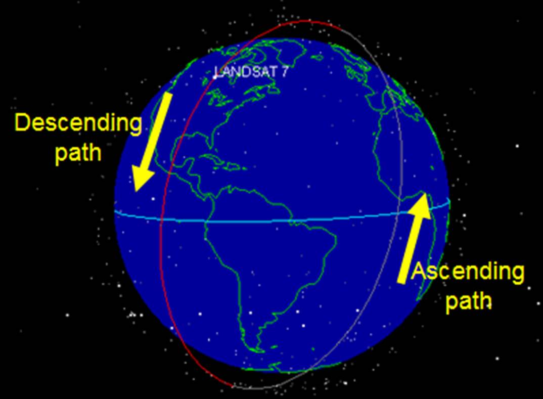
Figure 4. Ascending and descending paths
Sensor Geometry and Scene Referencing
Swath Width and IFOV
As shown in Figure 5, the swath width is the range imaged by a sensor in each swath. The instantaneous field of view (IFOV) is the solid angle through which a detector is sensitive to radiation. In a scanning system this refers to the solid angle subtended by the detector when the scanning motion is stopped. The IFOV is commonly expressed in milliradians. (Note: 1 rad = 1000 mrad). For example, the Thematic Mapper (TM) sensor in Landsat 4 & 5 (altitude: 705km) had the IFOV of 0.043 mrad for the bands 1,2,3,4,5 and 7 at nadir. The diameter on the ground can be calculated using [altitude x IFOV], where IFOV is in radian. In the case of the Landsat TM sensor, it is [705000 m X 0.000043 rad], which produces about 30 m. The pixel size of satellite imagery is frequently determined by the IFOV of the sensor.
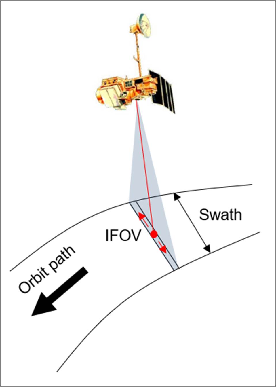
Figure 5. Swath and IFOV (Instantaneous Field of View)
Scanning Types
Two scanning types that are used by earth imaging satellites as shown in Figure 6. One is across-track scanning and the other is along-track scanning.
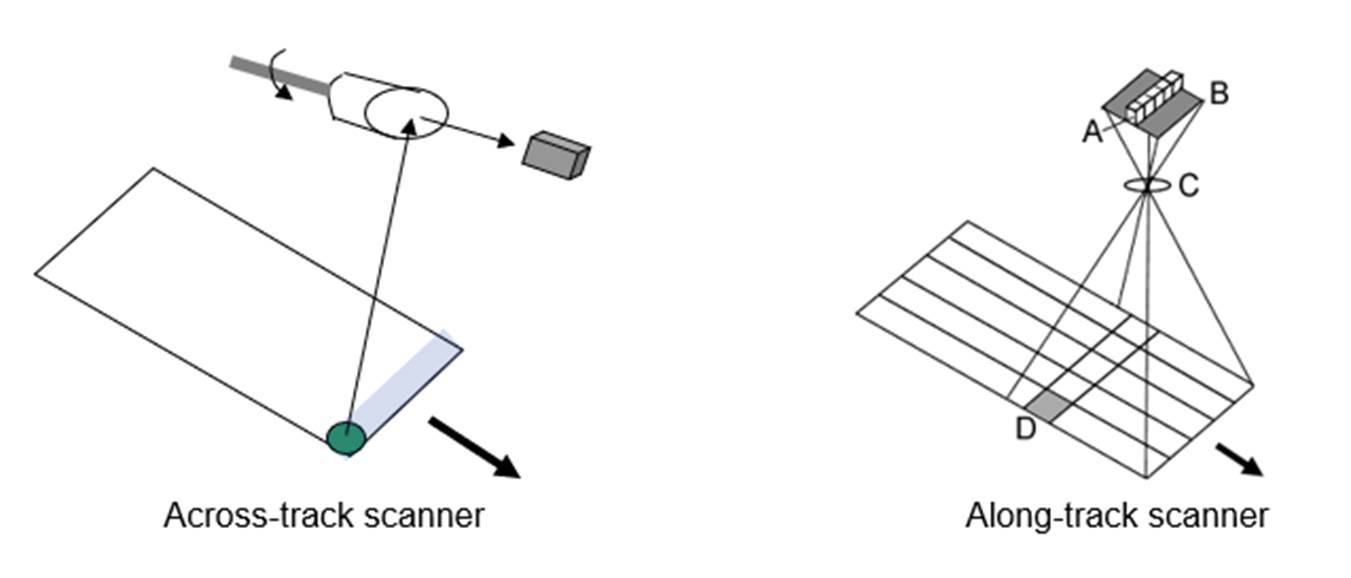
Figure 6. Across-track and along-track scanners.
Across-track scanners are also known as Whiskbroom scanners. Across-track scanners scan the Earth in a series of lines. The lines are oriented perpendicular to the direction of motion of the sensor platform. Each line is scanned from one side of the sensor to the other, using a rotating mirror. As the platform moves forward over the Earth, successive scans build up a two-dimensional image of the Earth’s surface. The incoming reflected or emitted radiation is separated into several spectral components that are detected independently.
Along-track scanners are also known as push broom scanners. Along-track scanners use the forward motion of the platform to record successive scan lines and build up a two-dimensional image, perpendicular to the flight direction. However, instead of a scanning mirror, they use a linear array of detectors located at the focal plane of the image formed by lens systems, which are "pushed" along in the flight track direction. Because push broom scanners carry more sensors, they require more calibration work than whiskbroom scanners.
Worldwide Reference System (WRS)
Continuously captured images along a swath are split into many scenes to facilitate referencing, archiving, and browsing. In the case of Landsat 1, 2, and 3 satellites, they used WRS-1 (World Referencing System – 1). WRS-2 is used with Landsat 4, 5, 7, and 8 satellite imagery. WRS uses path and row numbers to identify scene locations. The path number increases towards the west, and the row number increases towards the south.
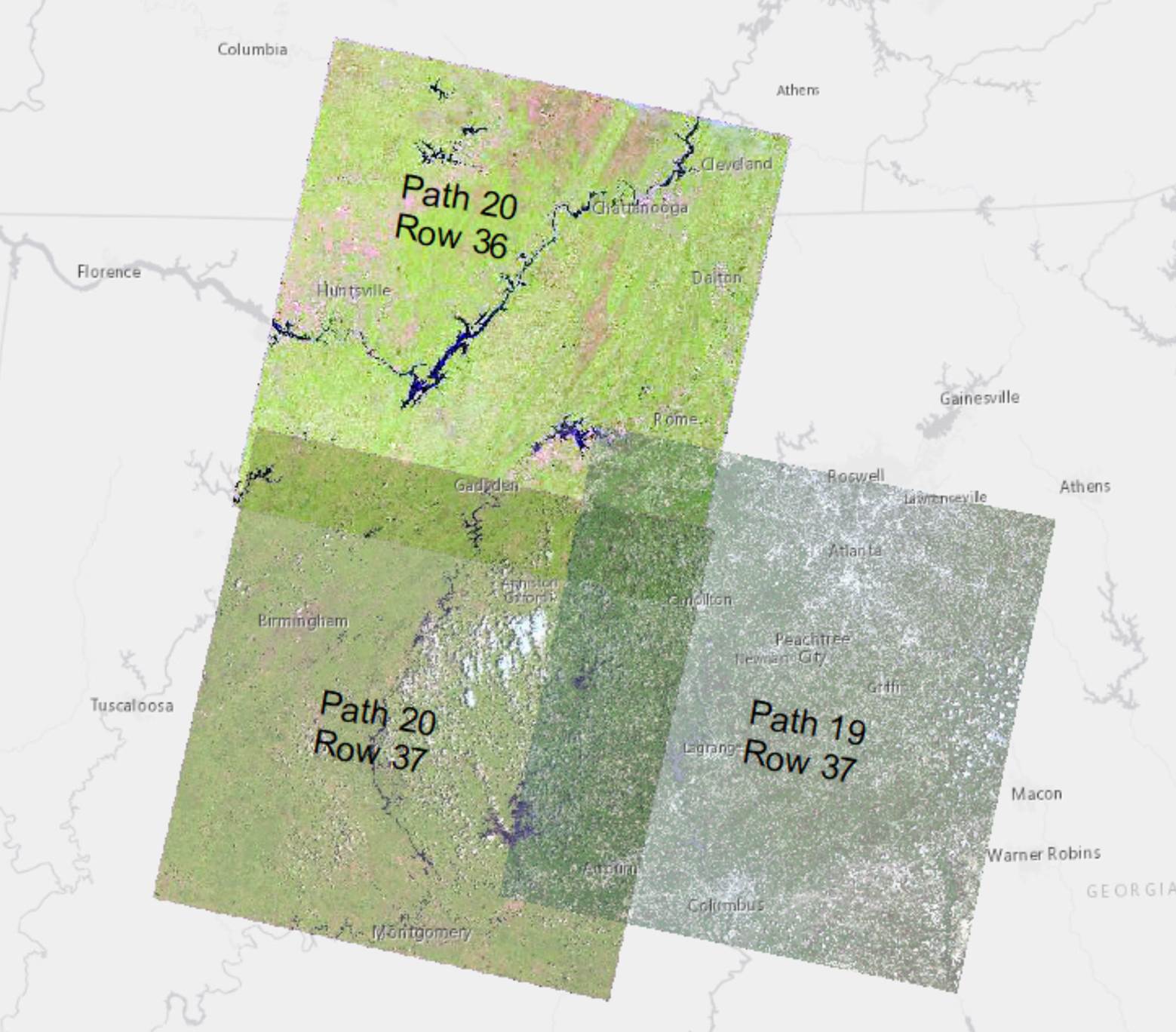
Figure 7. The path and row numbers of three Landsat 8 scenes. Atlanta and vicinity.
In the case of ARD (Analysis Ready Data) dataset, a different scene referencing system is used. ARD, recently developed by the USGS, is a fully processed dataset that can be applied for further analyses without pre-processing such as geometric and radiometric corrections. The ARD provides surface reflectance (SR), provisional surface temperature (ST), burned area (BA), fractional snow-covered area (FSCA), and dynamic surface water extent (DSWE) layers. ARD uses a grid to reference scene locations as shown in Figure 8. Figure 9 shows the ARD data search results using the EarthExplorer web application (https://EarthExplorer.usgs.gov), and the Atlanta and vicinity are referenced by H24 and V13.
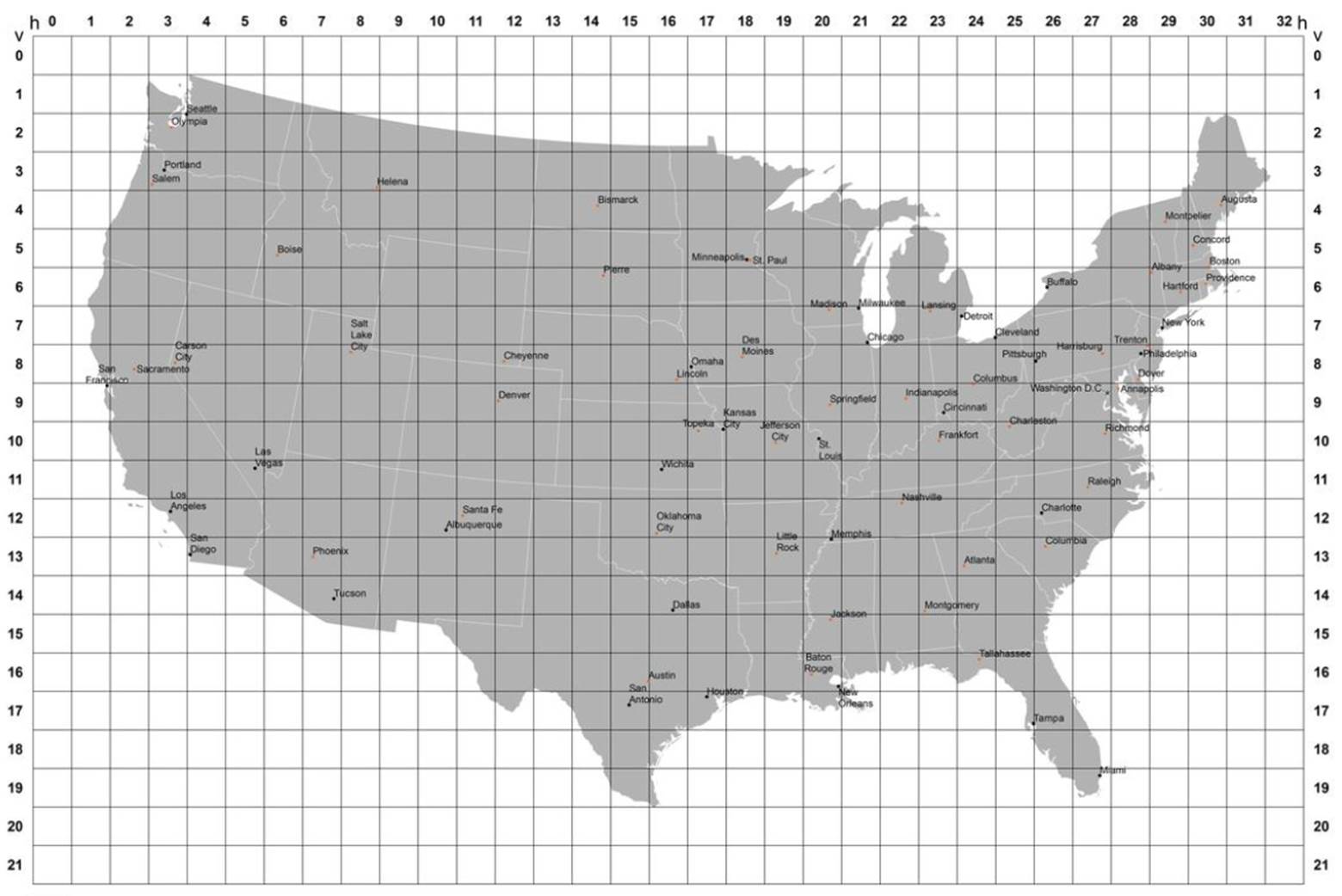
Figure 8. ARD grid referencing system for the conterminous U.S. (USGS, 2019)
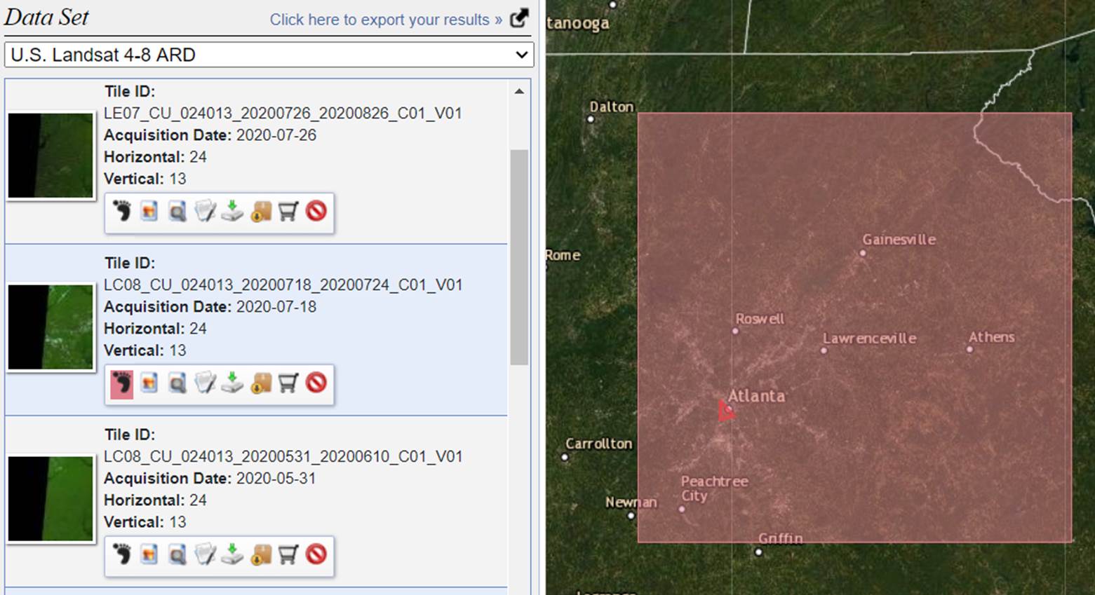
Figure 9. Example of the ARD referencing system. Atlanta and vicinity. URL: https://EarthExplorer.usgs.gov.
Landsat Satellites
The Landsat satellites are the most popular mid-resolution instruments because of their data archive since 1972 and the free-of-charge data download policy since 2008. Jointly managed by NASA and the U.S. Geological Survey, Landsat satellites have carried various sensors as shown in the following tables.
Sensors and Bands
Table 1. Landsat 1-5: Multispectral Scanner (MSS)
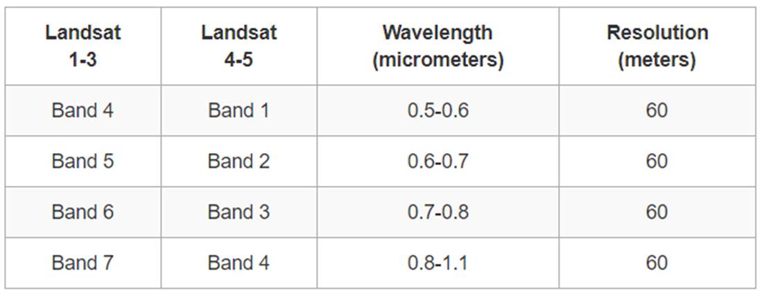
Table 2. Landsat 4-5: Thematic Mapper (TM)
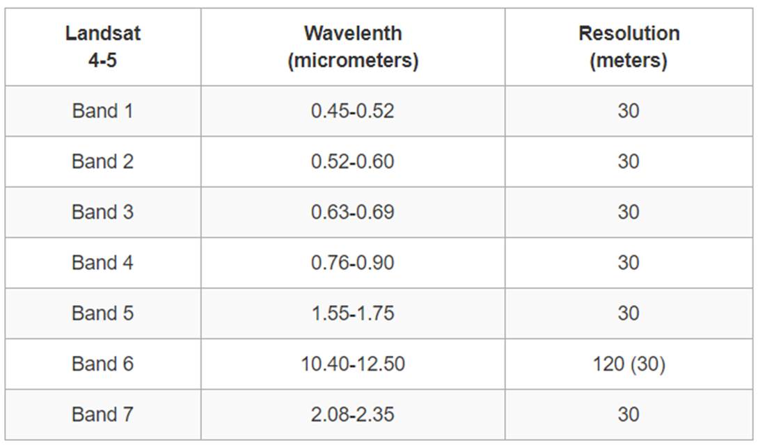
Table 3. Landsat 7: Enhanced Thematic Mapper Plus (ETM+)
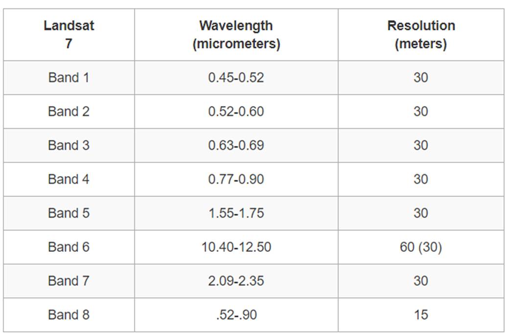
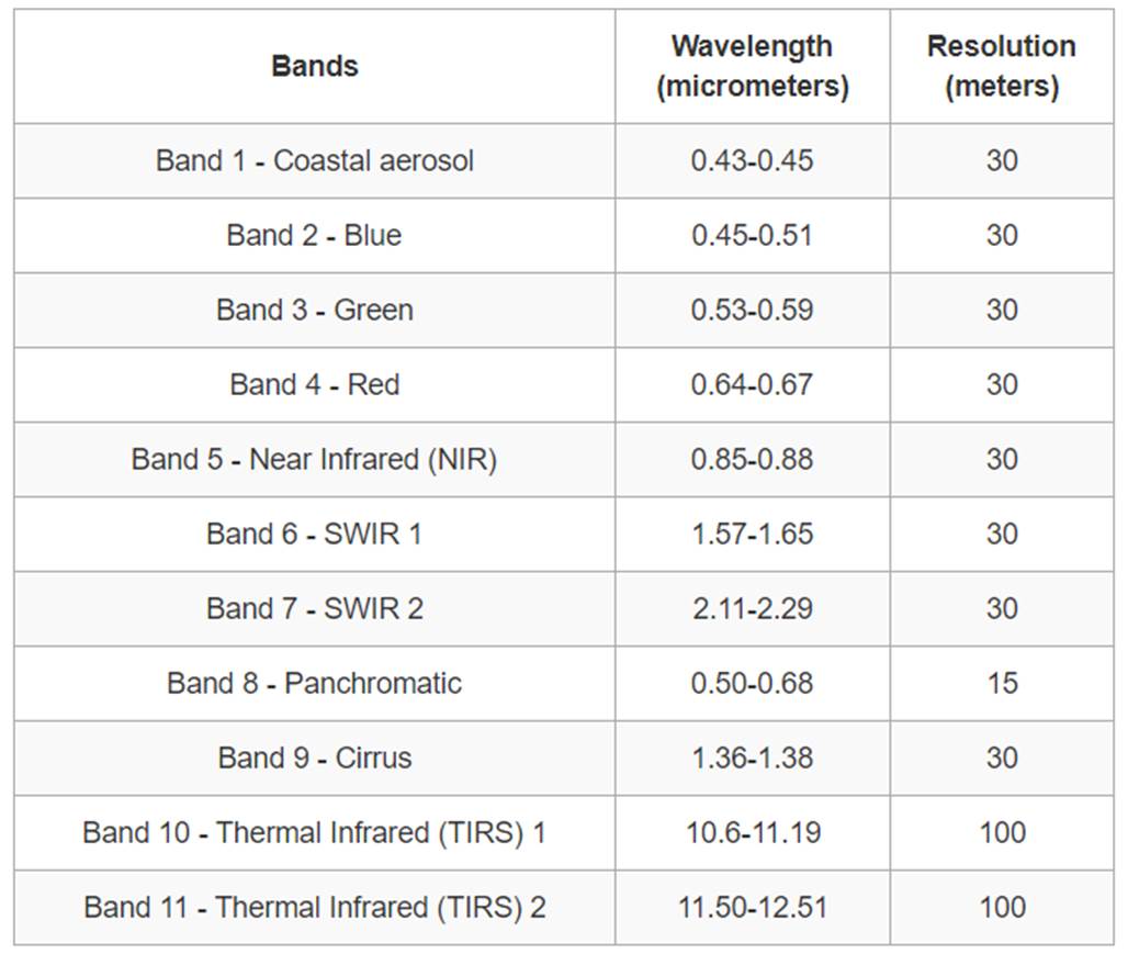
Table 4. Landsat 8: Operational Land Imager (OLI) and Thermal Infrared Sensor (TIRS)
Because the MSS sensor does not have a blue band, it is impossible to make a real color composite using the MSS data. Figure 10 shows a color infrared composite using the MSS data captured on April 20, 1976. Southern California.
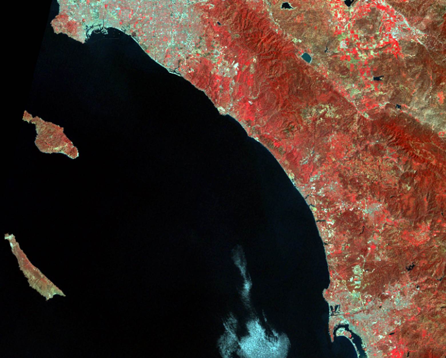
Figure 10. A CIR composite with Landsat MSS data. The reddish tone indicates vegetation. Southern California, 1976.
Panchromatic Band
Landsat 7 and 8 carry a panchromatic band. The band covers the visible wavelength range in one band. The panchromatic band provides a higher spatial resolution of 15m than other multispectral bands. Figure 11 shows the difference of spatial resolution between the 30 m multispectral bands and the 15 m panchromatic band of a Landsat 7 ETM+ sensor image.
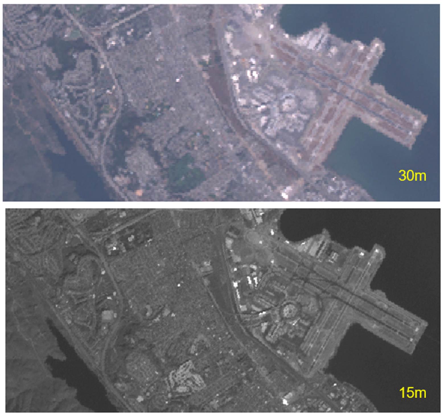
Figure 11. The 30 m multispectral band and the 15 m panchromatic band of a Landsat 7 ETM+ image. The image shows the international airport in San Francisco.
Coastal / Aerosol Band in OLI
The Landsat 8 OLI sensor detects the 0.433-0.453 µm wavelength range in band 1, and the band, a.k.a. coastal/aerosol band, is useful for imaging shallow water and tracking fine atmospheric particles like dust and smoke. The band reflects blues and violets and displays subtle differences in the color of water. The band has been used for monitoring chlorophyll concentrations and suspended sediments in the water, as well as phytoplankton and algae blooms. This band is also useful in tracking and estimating the concentration of fine aerosol particles such as smoke and haze in the atmosphere. Figure 12 shows a color composite using the OLI bands 6, 5 and, 1 for RGB colors, respectively.
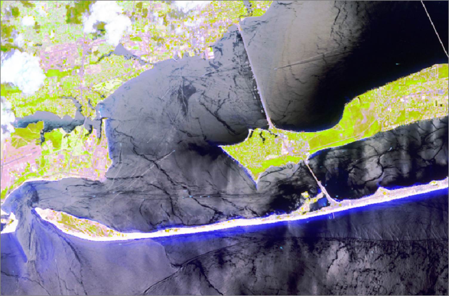
Figure 12. An example of using OLI band 1 (coastal/aerosol band) for a color composite. Pensacola, Florida. Landsat 8 OLI. Bands 6-5-1 for R-G-B, respectively.
MODIS Instrument Onboard Terra and Aqua Satellites
MODIS stands for Moderate Resolution Imaging Spectroradiometer. It provides comprehensive measurements of ocean life, land vegetation, cloud cover, and fires. MODIS is frequently used to monitor natural disasters covering large areas. The MODIS instrument provides high radiometric sensitivity in 12-bit quantization in 36 spectral bands ranging in wavelength from 0.4 µm to 14.4 µm. The responses are custom tailored to the individual needs of the user community and provide an exceptionally low out-of-band response. Two bands are imaged at a nominal resolution of 250 m at nadir, with five bands at 500 m, and the remaining 29 bands at 1 km. A ±55-degree scanning pattern at the 705 km altitude achieves a 2,330 km swath and provides global coverage every one to two days. Table 5 shows MODIS bands and their primary uses. Also, Figures 13 and 14 show the wildfires and dust storms imaged by MODIS.
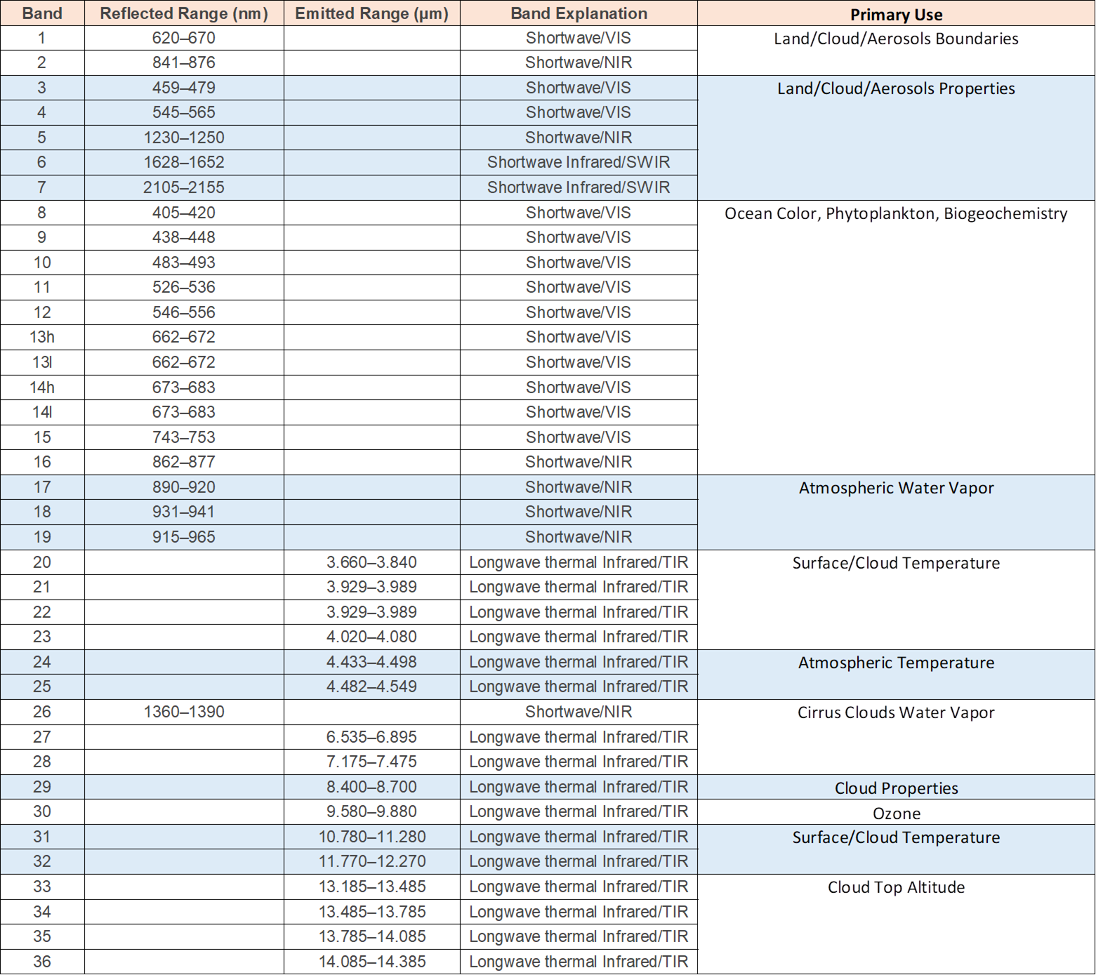
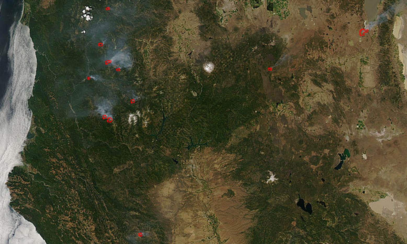
Figure 13. Wildfires captured by the MODIS sensor. Northern California, July 27, 2006. https://modis.gsfc.nasa.gov/
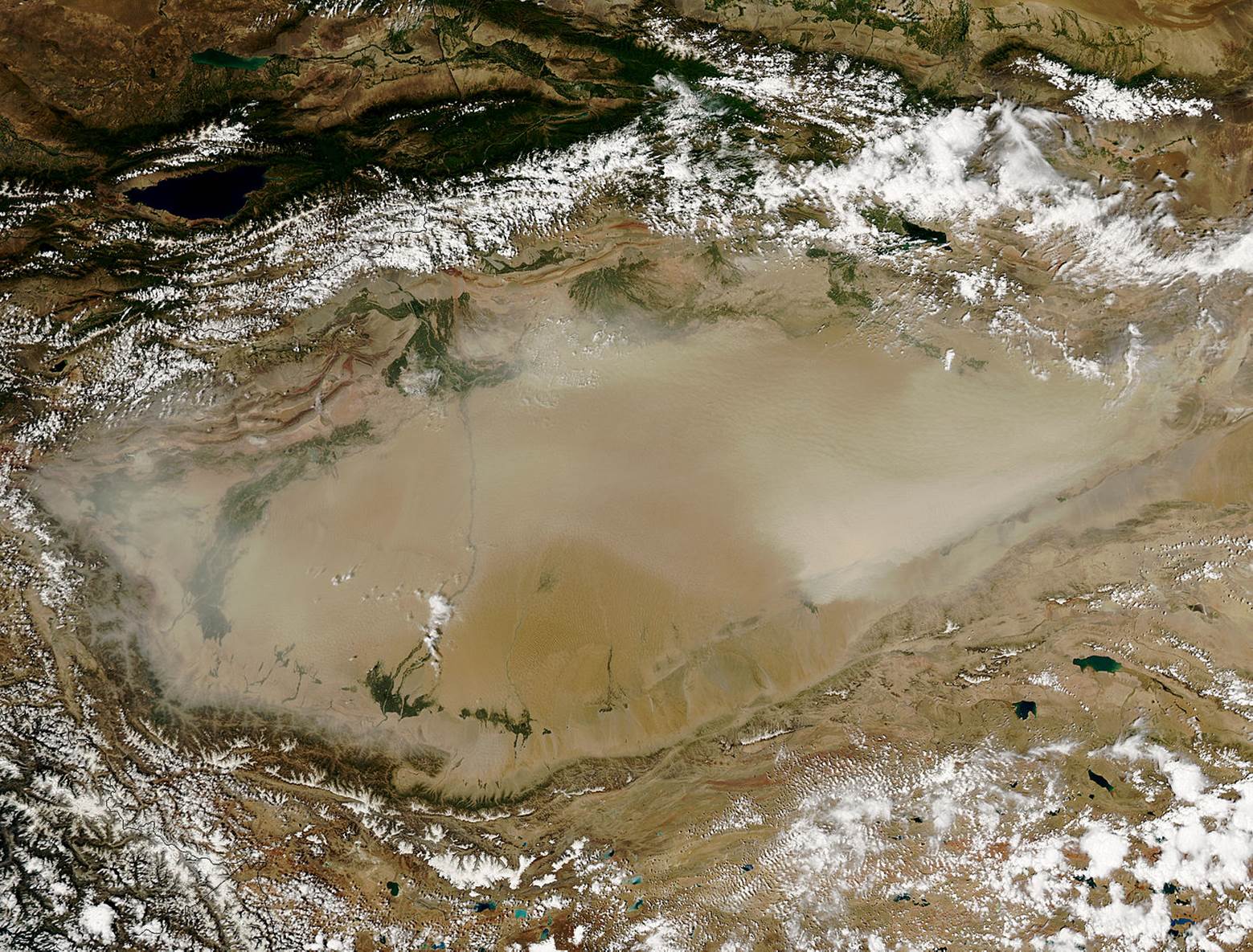
Figure 14. Dust storm captured by the MODIS sensor. The Taklimakan Desert in China, July 26, 2006. https://modis.gsfc.nasa.gov/
References
USGS, 2019. U.S. Landsat Collection 1 (C1) Analysis Ready Data (ARD) Data Format Control Book (DFCB). https://prd-wret.s3.us-west-2.amazonaws.com/assets/palladium/production/atoms/files/LSDS-1873_US_Landsat_C1_ARD_DFCB-v6.pdf