Chapter Contents
Handling remotely sensed imagery requires some knowledge about how image files are structured. In this chapter, we will look at some properties of digital imagery, file structures, file formats, and multiband image display.
Digital Image Properties
Image Structure
A digital image is composed of a set of numbers and metadata information about the numbers. Most remote sensing images represent a rectangular area, and the numbers fill the area in a regular grid pattern as shown in Figure 1.
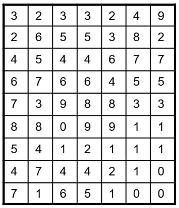
Figure 1. An imaginary digital image showing pixel values.
A pixel or cell is the base unit that constitutes an image. Each pixel represents a square area in most cases; however, it may represent a rectangular area or other shapes. In this example, there are 63 pixels.
Pixel size or cell size indicates the areal size of a pixel. However, interestingly, it is conventionally used for indicating the distance of an edge of a pixel instead of the actual areal size. Supposing a pixel represents 25 x 25 meters on the ground, people say, “The pixel size is 25m.”
Resolution indicates the level of detail of an image. As the pixel size decreases, the resolution increases. Specifically, this kind of level of spatial detail is called “spatial resolution.” A fine resolution image has more pixels than a coarse resolution image. In the case of a digital camera, more pixels will provide a finer resolution image.
The number of pixels along a column is called “the number of rows” or “lines.” “The number of columns” or “samples” indicate the number of pixels along a row. The product of rows and columns is the total number of pixels.
There are many ways of determining pixel values. Pixel values frequently represent reflectance levels. They may also represent other information such as quality flag values, land cover types, temperature, etc.
Quantization
Pixel values are mostly numbers, and there are many different number types such as binary, integers, and real numbers. Quantization indicates how many bits are used to write pixel values. If too many bits are used for quantization, computer memory and disk space may be wasted. On the contrary, if too little bits are used, the level of details will be lost.
The simplest quantization is to use 1-bit. The 1-bit quantization can represent either 0 or 1. The 1-bit quantization is called binary quantization.
The next quantization used frequently is the 8-bit quantization. In computer science, 8-bits make 1-byte. The 8-bit quantization can contain values ranging from 0 to 255. It has been used frequently in popular graphic image formats such as JPEG, TIFF, and BMP.
The unsigned short integer quantization uses 2-bytes which can represent 0 ~ 65,535. The signed short integer also uses 2-bytes, and it can represent -32,767 ~ 32,767. The signed, short integer is good enough to represent global elevation in meters without decimals.
The Integer quantization uses 4 bytes ranging from -2,147,483,648 to +2,147,483,648.
Real numbers can be quantized with either float or double formats. The float format uses the single-precision represented by 4 bytes. The double format uses the double-precision represented by 8 bytes. The double precision is good for representing geographic coordinates at very high precision.
Most imaging sensors quantize incident energy into 8-bit levels, i.e. 0-255. However, occasionally, more quantization levels are used in high-end professional consumer cameras and some imaging sensors onboard satellite. For example, the Landsat 8 OLI (Operational Land Imager) sensor uses 12-bit quantization, even if their processed products (ex. Landsat ARD Dataset) are delivered to end-users in the 16-bit integer format, i.e. the signed short integer quantization, as shown in Figure 2. The figure shows that the SRB1 band values are written with the ”INT16” format which is the signed short integer quantization method.
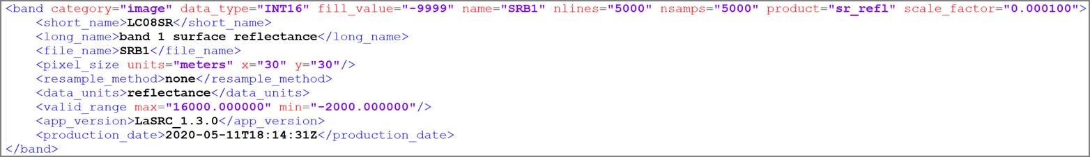
Figure 2. A portion of a Landsat 8 ARD (Analysis Ready Dataset) metadata.
Endian
Quantized pixel values may be written in the computer memory differently depending on what kind of CPU (central processing unit) the computer uses. Endian, a.k.a. byte order, means the method of writing a multi-byte number to a computer memory.
There are two endian types: big endian and little endian. The big endian writes a multi-byte number from the first byte, while the little endian writes from the last byte. Table 1 shows CPU processors and endian types. In the table, Bi endian indicates that both big and little endian types are used in a single processor. In this case, integers are written in little endian and real numbers are written in big endian. Identifying the endian used in an image, is very important when the image is processed with multiple platforms.
Table 1. CPU processors and endian types
|
Processor |
Endian Type |
|
Motorola 68000 |
Big Endian |
|
PowerPC (PPC) |
Big Endian |
|
Sun Sparc |
Big Endian |
|
IBM S/390 |
Big Endian |
|
Intel x86 (32 bit) |
Little Endian |
|
Intel x86 (64 bit) |
Little Endian |
|
Dec VAX |
Little Endian |
|
Alpha |
Bi (Big/Little) Endian |
|
ARM |
Bi (Big/Little) Endian |
|
IA-64 (64 bit) |
Bi (Big/Little) Endian |
|
MIPS |
Bi (Big/Little) Endian |
Bands
Digital imagery mostly comes with multiple reflectance bands. Each band covers a range of wavelengths. The Panchromatic band covers all the visible wavelengths (from violet to red).
Figure 3 shows the multispectral bands captured by MSI onboard Sentinel-2, OLI and TIRS onboard Landsat 8, ETM+ onboard Landsat 7, and ASTER and MODIS onboard TERRA and AQUA. In the case of Landsat 8, nine (9) bands are captured by the OLI sensor, and two (2) bands are captured by the TIRS thermal sensor. The MODIS sensor captures significantly more bands than other sensors. For example, there are three bands that capture the red band wavelengths. The range of wavelengths covered by a band is spectral resolution. The figure shows that the MODIS sensor has the finest spectral resolutions in most bands.
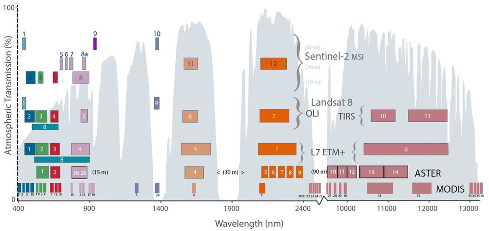
Figure 3. Multispectral bands captured by various imaging sensors.
Some imaging sensors capture numerous bands where bands are neighboring sequentially. That kind of sensor is, what we call, hyperspectral sensor. For example, the Hyperion sensor is a hyperspectral sensor. It was used in NASA's Earth Observing-1 (EO-1) spacecraft. The Hyperion sensor collected 220 spectral bands sequentially covering from 0.4 to 2.5 µm.
Unlike hyperspectral bands, multispectral bands are not contiguous so that there are gaps between multispectral bands.
Coordinates in an Image
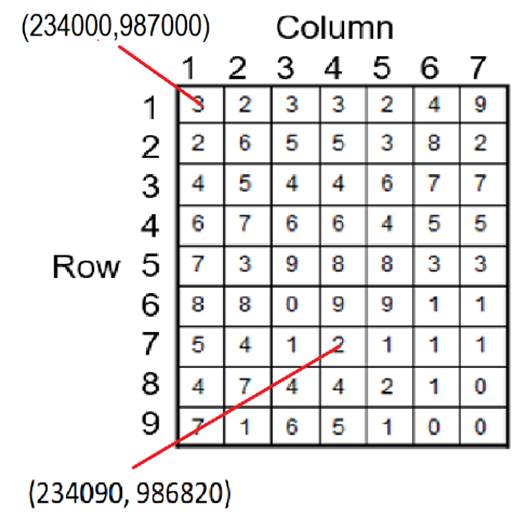
Coordinates are implicitly implemented in an image. Using the pixel size and the coordinates of a pixel, we can calculate the coordinates of other pixels. For example, suppose that a pixel size is 30m and the (x, y) coordinates of the upper left corner pixel are (234000, 987000) at the center of the pixel. Then, the coordinates of a pixel (at the center) in row 7 and column 4 will be (234090, 986820) as shown below:
y = 987000 - (Row – datumRow) x pixelSize
= 987000 - (7 – 1) x 30
= 9874000 – 180
= 986820
x = 234000 + (Column - datumColumn) x pixelSize
= 234000 + (4 – 1) x 30
= 234000 + 90
= 234090
File Structure
Body and Metadata
Most image files consist of pixel values and metadata information. An image file’s main Body carries pixel values. Metadata information may contain the number of rows, number of columns, quantization method, coordinates of the image corners, pixel size, color lookup table, projection information, byte order, imaging date and time, imaging device, agency information, and image processing information. The metadata information may be written in a separate file, or it may be a part of an image file. In the case of the JPEG file format, the metadata information is written inside a JPEG file. Most satellite imagery, however, comes with a separate metadata file(s).
Writing Multiple Bands in a File
There are three major methods of writing multiple bands in a file as shown in Figure 4. One method is to write bands sequentially, as known as the band sequential (BSQ) method. In the BSQ method, one band is written completely, and the next band follows.
Another method is to interleave bands by lines, also known as band-interleaved by line (BIL) method. In this method, multiple bands are interleaved line by line.
Another method is to interleave bands by pixels, also known as band-interleaved by pixel (BIP) method. In this method, multiple bands are interleaved pixel by pixel. The BIP is good for fast display so that it is used by many famous digital image formats such as JPEG and TIFF.
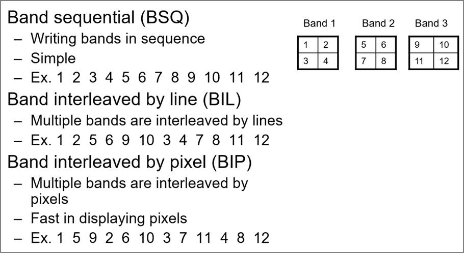
Figure 4. Three different methods of writing multi-bands in a file.
Color Look-up Table
An image file may contain a color lookup table. The color lookup table defines how to represent each pixel value. For example, in Figure 5, pixel value “1” is represented as red supposing each color ranges from 0 to 255.
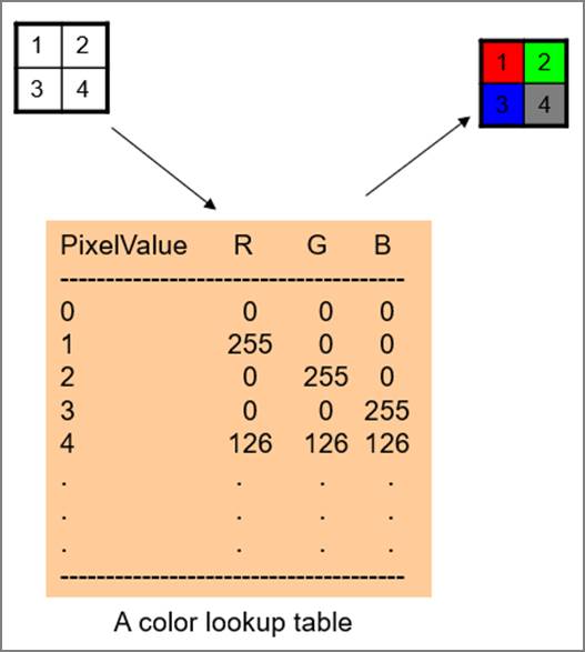
Figure 5. An example of using a color look-up table.
The GIF file format is a typical example of using a color lookup table. It is very good for representing non-photographic data such as rasterized vector maps. With photographic data, however, the color lookup table will be very long to represent millions of colors, resulting in inefficiency. The GIF format was applied in the USGS scanned topographic maps, such as the Digital Raster Graphic (DLG) dataset.
Pyramid Layers
An image file may also contain pyramid layers as an embedded object or an auxiliary file. Pyramid layers mean the multiple, reduced-resolution image layers that are created by resampling pixels from the original image, as shown in Figure 6. The reduced-resolution layers are used to speed up image display on monitors. Without pyramid layers, each display operation such as zooming or panning would invoke direct access to its original image to resample pixel values to display on a screen, which may take a long time with a large image file. However, once pyramid layers are constructed, pixel values are read without resampling pixels.
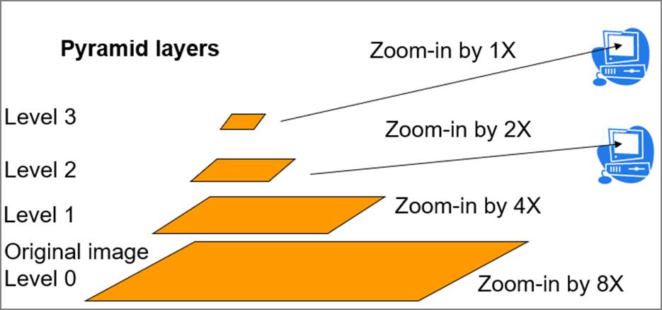
Figure 6. Pyramid layers.
Image File Formats
There are many image file formats, and one way of grouping them consider how many concurrent users they support. The local image file formats support only one user at a time, while the enterprise server system supports multiple concurrent users. The following lists some local formats and enterprise systems.
· Local file formats
o GeoTIFF: The GeoTIFF is a local image file format. It uses “.tif” as the file extension. It extends the traditional TIFF format by adding more tagged metadata to the file like geographic coordinates and projection information. For example, it is used to archive the Landsat satellite imagery.
o HDF: The HDF (Hierarchical Data Format) has been used to archive the images obtained by NASA’s earth-observing satellites. It uses “.hdf”, “.hdf4”, or “.hdf5” as the file extension. HDF is organized into instances of zero or more groups or datasets, together with supporting metadata. Each group or dataset is organized into a multidimensional array of data elements, together with supporting metadata.
o IMG: The IMG is a proprietary file format by ERDAS Imagine. It uses “.img” as the file extension.
o GRID: The GRID is a proprietary file format by Esri ArcGIS. It does not use a file extension. Instead, a folder is used to organize an image.
· Enterprise server systems
o Web Map Service: Developed by Open Geospatial Consortium (OGC).
o ArcGIS Server: Developed by Esri.
Compression Formats
Image files are mostly voluminous, and they are frequently compressed to save computer memory space and to reduce data delivery volumes. There are two types of compression algorithms -- lossless compression and lossy compression. The lossless compression method keeps all original pixel values, but the lossy compression methods sacrifice original pixel values slightly to achieve a higher compression ratio. Compressed images files can be identified by their file extensions. The following lists the compressed file types that are commonly used with remote sensing images:
· Lossless compression
o .zip : Most frequently used format
o .gz : GNU Zip
o .7z : Opensource file format
· Lossy compression
o .jpg : JPEG
o .jp2 : JPEG 2000
o .sid : A proprietary compressed image file format.
Even if it is not a compression file type, the TAR file type is also frequently used in remote sensing. It has “.tar” as the file extension. The TAR format is used to archive multiple files and folders into one TAR file. For example, “LC08_L1TP_019037_20200506_20200509_01_T1.tar.gz” is a Landsat 8 scene downloaded from the USGS. The “.tar.gz” extension in the name indicates that the image was first archived into a tar file and then compressed into a gz file. In order to use the file, users will need to unzip the gz compression, and then unzip the tar archive one more time.
Displaying Imagery
With One Band
With a one-band image, we can use the grayscale or the pseudo-color display method as shown in Figure 7. The gray-scale display method stretches original pixel values to the 0~255 gray-scale. Zero (0) is usually black and 255 is white.
The pseudo-color display method uses a color lookup table. The color lookup table, also known as color ramp, tells how each pixel value should be displayed. The figure shows an example of a color lookup table, which uses a rainbow color scheme. Value 0 is represented as purple, and Value 255 as red.
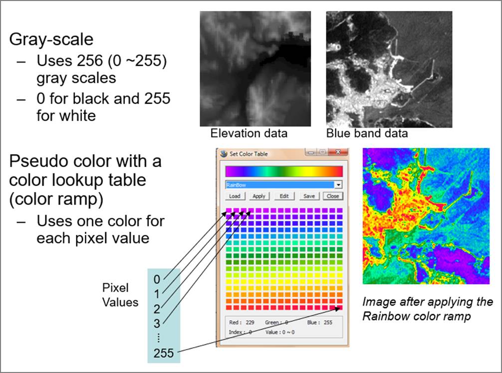
Figure 7. Visualization of one band image
With Multiple Bands
If an image has multiple bands, it may be used to create color composites. To create a color composite, three bands are needed because color displays use red, green and blue (RGB) elements to make colors.
Depending on which bands are assigned to RGB, two composite types exist: real color composite and false color composite. The real color composite assigns the red, green and blue wavelength bands to R, G, and B, respectively, making the same colors as our eyes see. All other band assignments for RGB produce false color composites.
Figure 8 shows a real color composite and false color composites of the San Francisco Bay area. Image A is a real color composite where red, green, and blue bands were used for RGB, respectively. Image B is a false color composite. It uses far infrared, near-infrared, and red bands for RGB. Image C is another false color composite, which uses near-infrared, red, and blue bands for RGB. Image C shows a very good characterization of vegetation in reddish colors.
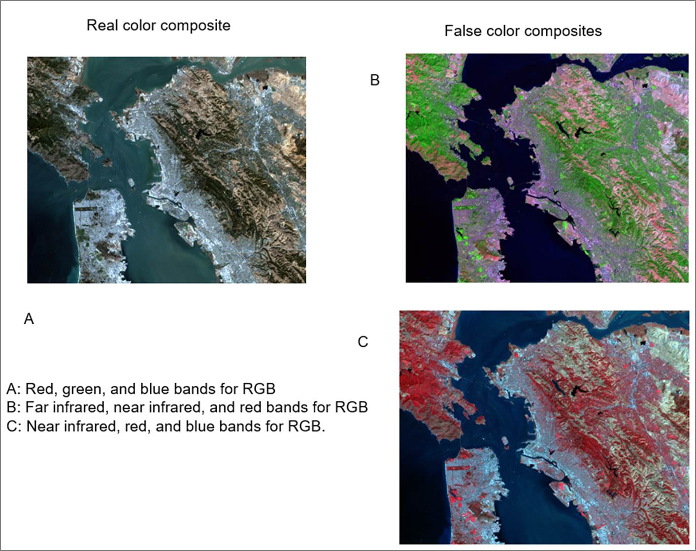
Figure 8. Color composite examples with a Landsat multi-band image.