Chapter Contents
Land Surface Emissivity (LSE) Models for Landsat Imagery
Temperature Calculation with Landsat Imagery
Introduction
Temperature is a very significant parameter that is used for monitoring the biosphere, hydrosphere, atmosphere, and even lithosphere. In situ measurements are expensive and time-consuming, while thermal remote sensing provides relatively inexpensive and fast temperature measurements. Most visible, near-infrared, and microwave sensors detects reflected energy. Thermal sensors, however, are used to detect the temperature of objects using the energy emitted from objects.
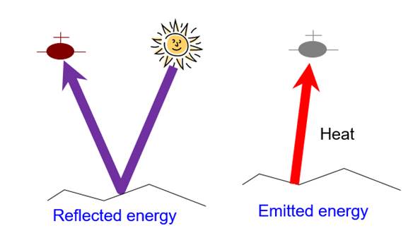
Figure 1. Reflected vs. emitted energy
The amount of energy emitted from an object is dependent on the temperature of the object. According to the Stefan-Boltzmann Law, the total amount of radiance energy increases as the temperature of an object increases. In the case of an imaginary blackbody, which absorbs and emits the full amount of radiative flux, its radiance is proportional to the fourth power of temperature as shown below.
![]() [Eq. 1] Stefan-Boltzmann Law (Blackbody)
[Eq. 1] Stefan-Boltzmann Law (Blackbody)
Where,
J is the total energy radiated per unit surface area of a black body across all wavelengths per unit time, frequently measured as watts per square meter (![]() ), c is the Stefan-Boltzmann Constant of 5.6697 x 10⁻⁸ W m-2 K-4, and T is the absolute temperature measured in Kelvin degrees.
), c is the Stefan-Boltzmann Constant of 5.6697 x 10⁻⁸ W m-2 K-4, and T is the absolute temperature measured in Kelvin degrees.
Emissivity
A black body is an imaginary object. In the real world, every object does not emit the full amount of incident energy. Such object is called a graybody. It emits only a fraction of the radiation emitted by a blackbody at the equivalent temperature. The fraction is called emissivity (e) as shown in [Eq. 2]. The emissivity values may range from 0.0 to 1.0. A blackbody has an emissivity of 1.0.
![]() [Eq. 2]
[Eq. 2]
Where,
e is emissivity, and λ is wavelength. The subscript λ indicates that emissivity is dependent on wavelength, as shown in Figure 2.
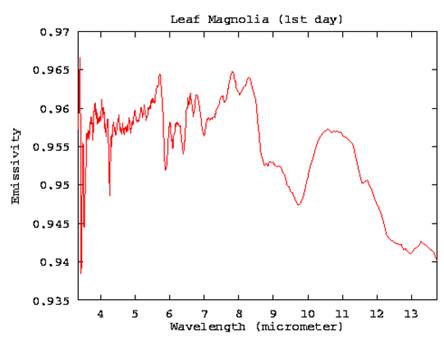
Figure 2. Emissivity vs. Wavelength (Ex. Magnolia)
Considering emissivity (e), the total radiation of a real-world object becomes:
![]() [Eq. 3] Stefan-Boltzmann Law (Graybody)
[Eq. 3] Stefan-Boltzmann Law (Graybody)
The emissivity values of real-world objects are also affected by mineral elements and water contents. In the case of water, ice, and snow, they generally have a high emissivity, 0.94 to 0.99, across the thermal infrared region. Interestingly, snow is unusual in that it has a high reflectance in the visible region where most of the incident energy is during the day, and a very high emissivity in the thermal region, resulting in snow being cold. Figure 3 shows the emissivity of various earth objects.
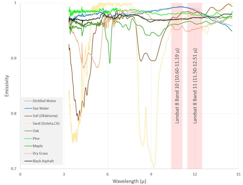
Figure 3. Emissivity of various objects. (Source data: http://www.icess.ucsb.edu/modis/EMIS/html/em.html)
Land Surface Emissivity (LSE) Models for Landsat Imagery
Multiple approaches have been developed to estimate land surface emissivity to work with satellite imagery. According to Sekertekin and Bonafoni (2019), there are three types of LSE models:
· Semi-empirical models
o Classification-based models
o NDVI-based models
· Physically-based models, and
· Multi-channel temperature/emissivity separation models
The last two models are not operational for Landsat data to obtain LSE due to the limitations presented in many studies, such as the requirement of more than two TIR bands or nighttime images. The semi-empirical models are used frequently with Landsat imagery. Particularly, NDVI-based models are popular because they are easy to implement and relatively satisfactory in results.
There are many NDVI-based emissivity models proposed. For example, Griend and Owe (1993) proposed a simple model, [e = 1.0094 + 0.047 ž ln(NDVI)]. According to Sekertekin and Bonafoni (2019), the RMSE (root mean square error) of the Griend and Owe model was about 5 Kelvin degrees. Another, more sophisticated model was proposed by Sobrino et al. (2008) as follows, and its RMSE was about 2.4 Kelvin degrees, according to Sekertekin and Bonafoni (2019).
![]()
[Eq. 4] Sobrino et al. model
Where,
R is the reflectance value of the red band, and P is the fractional vegetation cover calculated as:
P = [(NDVI – NDVImin) / (NDVImax – NDVImin)]2
Temperature Calculation with Landsat Imagery
Brightness Temperature vs. True Temperature
The brightness temperature is a descriptive measure of radiation in terms of the temperature of a hypothetical blackbody emitting an identical amount of radiation at the same wavelength. The brightness temperature is obtained by applying the inverse of the Planck function to the measured radiation.
Normally when we refer to temperate, we are referring to the kinetic temperature. Kinetic temperature or heat is generated by the vibration of molecules in all objects. Kinetic temperature is sometimes called true temperature. Kinetic temperatures can be measured using a thermometer and is measured using conventional temperature scales (°F,°C, K). There is a high correlation between the true temperature and brightness temperature. Therefore, we can utilize remote sensing technology to measure brightness temperature and correlate it to the true temperature.
Brightness Temperature Calculation
The pixel values of the Landsat thermal bands can be converted to the top-of atmosphere brightness temperature as follow:
· Convert pixel values to radiance values: Landsat imagery are provided to yours with various processing levels and algorithms. In the case of Landsat Level-1 imagery, pixel values can be converted to radiance values using the following equation, where DN indicates a pixel value:
Radiance (L) = Gain x DN + Offset
For the gain and offset values, refer to Landsat Data Users Handbook, ex. https://www.usgs.gov/media/files/landsat-8-data-users-handbook), and the metadata file that comes with each dataset.
· The second step is to convert the radiance values to the top-of-atmosphere brightness temperature values. The equation is as follow:
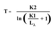
Where,
T is top-of-atmosphere brightness temperature.
Lλ is the radiance value of Band λ.
K1 is the band-specific thermal conversion constant (K1_CONSTANT_BAND_X) found in the metadata
K2 is also the band-specific thermal conversion constant (K2_CONSTANT_BAND_X) found in the metadata
K1 and K2 values for Landsat 5, 7, and 8 are as follows:
|
Landsat |
Band |
K1 |
K2 |
|
5 |
Band 6 |
607.76 |
1260.56 |
|
7 |
Band 6 |
666.09 |
1282.71 |
|
8 |
Band 10 |
774.8853 |
1321.0789 |
|
Band 11 |
480.8883 |
1201.1442 |
(Note: Data for Landsat 5 and 7 are from https://landsat.gsfc.nasa.gov/wp-content/uploads/2016/08/Landsat7_Handbook.pdf, and the data for Landsat 8 are from the Landsat Scene ID of LC80190362020127LGN00.
Land Surface Temperature (LST) Calculation
Due to various emissivity values and atmospheric interactions, the true temperatures of land surface features are different from their brightness temperatures. There are four major algorithms to calculate land surface temperature:
· mono window algorithm
· single-channel algorithm
· radiative transfer equation method, and
· split-window algorithm (SWA).
The first three algorithms can be used with one thermal band. The SWA, however, requires at least two thermal bands. The TIRS sensor onboard Landsat 8 provides two thermal bands so that SWA may be used with Landsat 8 imagery. For the first three algorithms, please refer to the paper by Sekertekin and Bonafoni (2019). A practical SWA proposed by Du et al. (2015) estimates land surface temperature with Landsat 8 TIRS bands as follow:

Where,
Ti = top of atmosphere brightness temperature for TIRS Band 10
Tj = top of atmosphere brightness temperature for TIRS Band 11
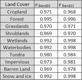
ε = the average emissivity of two bands, i.e. [0.5 x (εBand10 + εBand11)]. The emissivity values of common land cover types are as follows:
Δε = emissivity difference between two bands, i.e. [εBand10 - εBand11]
bk = coefficients as described below
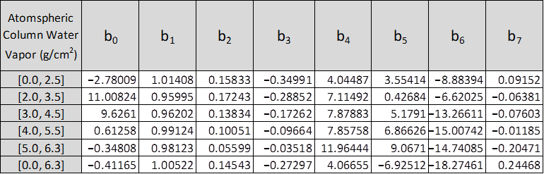
The amount of atmospheric column water vapor can be downloaded from the NASA Earth Observations (NEO at https://neo.sci.gsfc.nasa.gov/), as shown in Figure 4.
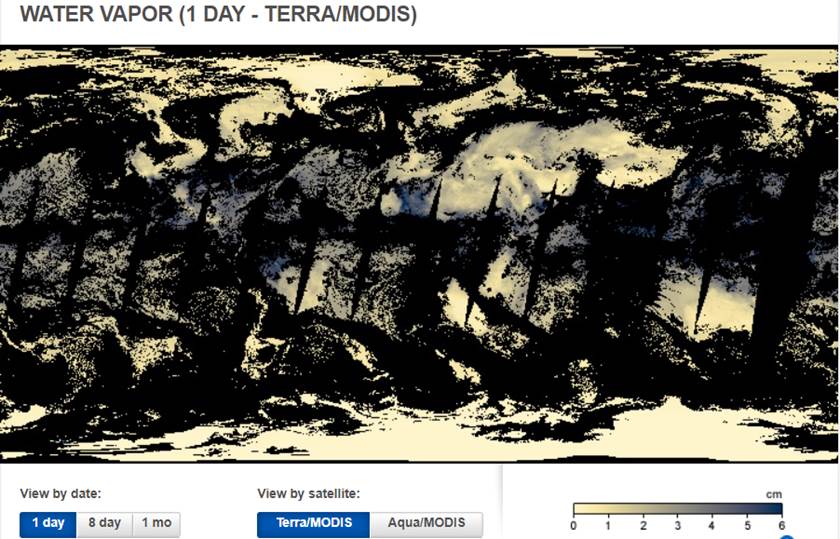
Figure 4. Atmospheric column water vapor. Note that the unit in this figure is cm, and the atmospheric column water vapor amount for bk in the model is g/cm2. They are the same because [g = cm3], so that the NEO’s water vapor amount can be used for the model without further conversion.
Thermal Imaging Applications
Thermal imaging has been applied to various application fields. Examples include surface temperature detection, camouflage detection, fire detection and fire risk mapping, evapotranspiration and drought monitoring, estimating air temperature, oil spill monitoring, water quality monitoring, volcanic activity monitoring, and urban heat island analysis.
Weather Applications
Thermal remote sensing is a very important method to collect weather data. Figure 5 shows the clear sky brightness temperature imaged by the GOES satellite. (Source: https://cimss.ssec.wisc.edu/goes/rt/viewdata.php?product=csbt_g11).
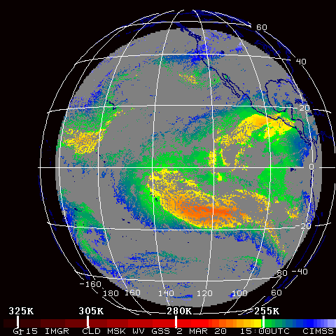
Figure 5. Clear sky brightness temperature
Figure 6 is another example that shows sea surface temperature created with images from NOAA satellites. (https://www.ospo.noaa.gov/Products/ocean/cb/sst5km/)
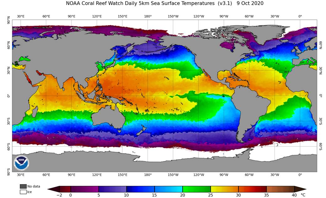
Figure 6. Sea surface temperature (SST)
Figure 7 shows another example of MODIS-derived land surface temperature. (Source: https://worldview.earthdata.nasa.gov/)
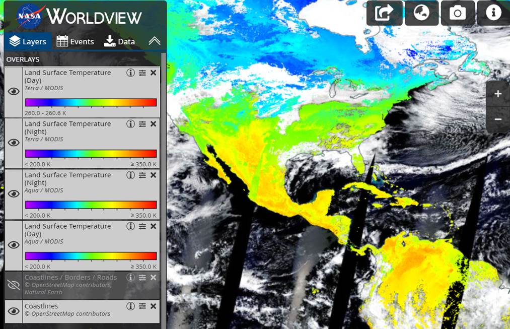
Figure 7. Land surface temperature.
Urban Heat Islands
Thermal images have been used to research urban heat islands. This thermal color-enhanced image, i.e. Figure 8, over the Atlanta central business district shows heating characteristics for various kinds of land cover types typical of urban areas, such as buildings, pavement and impervious surfaces, and vegetation. During the daytime air temperatures were in the low eighties and remotely sensed surface temperatures ranged from approximately 70 to 131 degrees Fahrenheit. The image shows surface heating across the urban landscape with a graduated color scale. White to red to orange are the warmest areas and yellow to green to blue the coolest. The white and red building roofs downtown are the hottest surface areas. The blue areas depict several cool areas downtown because of building shadows and forest areas in the southeast portion of the image. Yellow and green areas indicate temperature differentials between the surface and elevated roadways.
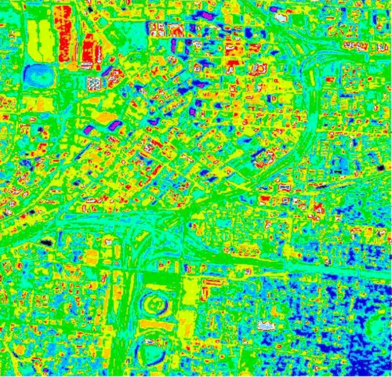
Figure 8. Landsat thermal image of Atlanta the downtown area.
Temperatures in an urban area are frequently compared with vegetation indices such as NDVI. Figure 9 shows a strong negative relationship between NDVI and land surface temperature measured from a Landsat 8 imagery taken on May 14, 2017, covering Atlanta and vicinity.
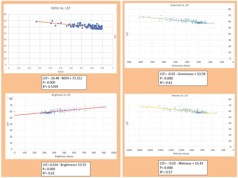
Figure 9. Land surface temperature vs. NDVI.
Archaeological Application
The images below, Figure 10, shows two false-color composites of TIMS data. The Chacoan roads are the linear features fanning out from the lower right-hand corner. The yellow lines are current day roadways. The current roads follow the topography and the path of least resistance in construction. Conversely, the prehistoric roads are strikingly linear. (Source: https://weather.msfc.nasa.gov/archeology/chaco_compare.html)
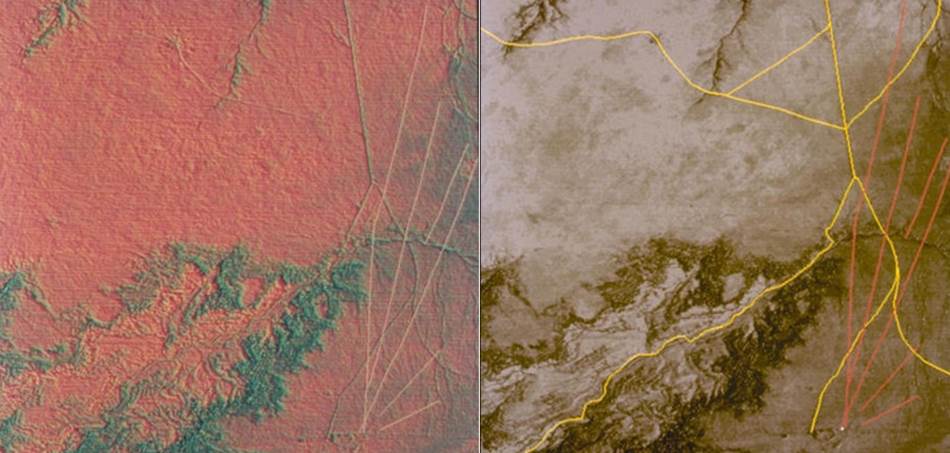
Figure 10. Fossil roads in the Chacoan desert.
Drought Monitoring
Temperature and precipitation datasets are some of the most important types of data used for drought and climate analysis. Temperature and precipitation data are collected from weather stations, weather radar, satellite and computer models. Early warning systems and drought monitoring tools are essential to manage the impact of water scarcities and minimize drought losses. While precipitation is considered the best observed hydrologic variable, scientists also use satellite sensors to monitor the land surface. Remote sensing data are important because there are useful drought-indicating parameters besides precipitation that can be measured from space, including evapotranspiration (ET), vegetation indices, land surface temperature (LST), and soil moisture. Figure 11 shows the evapotranspiration patterns captured from the MODIS sensor onboard the Terra satellite.
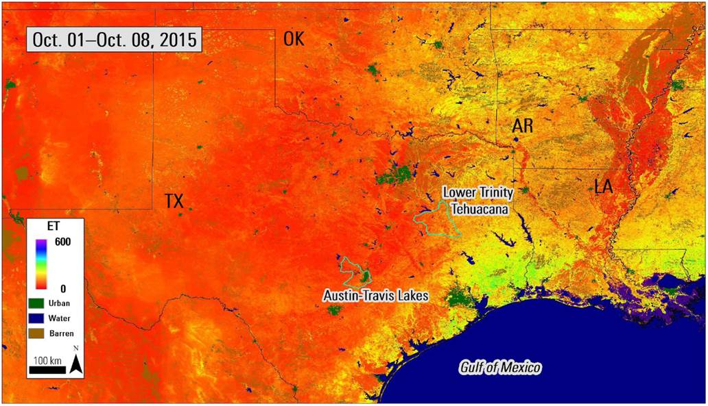
Figure 11. Terra MODIS 500-meter Evapotranspiration 8-day composite (MOD16A2.006) from October 01-08, 2015, over Texas and the south central United States. Source: https://lpdaac.usgs.gov/resources/data-action/two-sensors-are-greater-one-observing-drought-smap-and-modis/.
References
Du, C., Ren, H., Qin, Q., Meng, J., and Zhao, S., 2015. A Practical Split-Window Algorithm for Estimating Land Surface Temperature from Landsat 8 Data. Remote Sens. 2015, 7(1), 647-665; https://doi.org/10.3390/rs70100647. https://www.mdpi.com/2072-4292/7/1/647.
Griend, A. and Owe, M. 1993. On the relationship between thermal emissivity and the normalized difference vegetation index for natural surfaces. Int. J. Remote Sens. 14, 1119–1131.
Sekertekin, A. and Bonafoni, S. 2019. Land Surface Temperature Retrieval from Landsat 5, 7, and 8 over Rural Areas: Assessment of Different Retrieval Algorithms and Emissivity Models and Toolbox Implementation. Remote Sens. 2020, 12, 294; doi:10.3390/rs12020294. https://www.mdpi.com/2072-4292/12/2/294/htm
Sobrino, J.A., Jimenez-Muoz, J.C., Soria, G., Romaguera, M., Guanter, L., Moreno, J., Plaza, A., Martinez, P. 2008. Land surface emissivity retrieval from different VNIR and TIR sensors. IEEE Trans. Geosci. Remote Sens. 46, 316–327.