Chapter Contents
Side-looking Radar (SLR) Imaging
Introduction
The microwave region of the spectrum covers wavelengths from approximately 1mm to 1m. Microwaves are capable of penetrating the atmospheric features such as haze, light rain, light snow, clouds, and smoke so that microwave remote sensing is not affected by most atmospheric conditions.
Radar stands for radio detection and ranging and is a system that uses microwave energy for object detection and ranging. Here, ranging means measuring distance. Most Microwave sensors are active sensors, which means that they emit energy from an antenna and record the energy returned to the antenna. Passive sensors do not emit energy. Typical examples of passive sensors are Landsat OLI/TIRS and MODIS.
Radar Systems
Radar has been used to identify the range, altitude, direction, or speed of both moving and fixed objects such as aircraft, ships, motor vehicles, weather formations, and terrain. Three kinds of radar systems are popular – Doppler radar, plan position indicator, and side-looking radar. Doppler radar has been used for detecting speed. Plan position indicator (PPI) uses radial sweep on a circular display screen. PPI is popular in weather forecasting, air traffic control, and navigation applications. Side-looking radar (SLR) has been used for imaging land and ocean. SLR is the focus of this chapter. If SLR is equipped on an airplane, it is called SLAR (side-looking airborne radar).
Radar Frequencies and Major Applications
Table 1 shows different microwave wavelengths (bands) and their names. Radar bands are named Ka, K, Ku, X, C, S, L, and P as wavelength increases. The X and C bands are frequently used for SLR imaging. Longer wavelengths (i.e. 6cm or longer) are used for detecting soil moisture content, geology, and ocean waves. Shorter wavelengths (i.e. less than 3cm) are used for detecting wind, ice, geoid, vegetation, snow, and clouds. Table 2 shows wave lengths and target application areas.
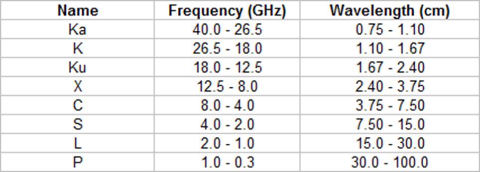
Table 1. Radar bands and their names.
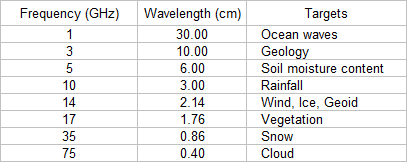
Table 2. Radar bands and their application areas.
Radar Imaging Satellites
Radar imaging has been used for many applications. During the 60s and 70s, radar imaging was used to map the areas that were covered by persistent clouds such as Panama, Amazon, and Venezuela. Since the 80s, space-borne radar imaging systems have become popular including Shuttle Imaging Radar (SIR), Almaz-1, ERS-1, JERS-1, SRTM, Envisat, Radarsat, KOMPSAT, and Sentinel-1.
The Sentinel-1 program has collected radar imagery since 2014, and Sentinel-1 data are freely available to the public (https://scihub.copernicus.eu/). The Sentinel-1 is a Copernicus Programme conducted by the European Space Agency. As of September 13, 2020, the Sentinel-1 programs have two satellites, Sentinel-1A and Sentinel-1B, which share the same orbital plane. They carry a C-band synthetic-aperture radar instrument.
Side-looking Radar (SLR) Imaging
SLR Geometry
SLR has been the major instrument for radar imaging of Earth’s surface. Understanding the geometry of SLR imaging is crucial for interpreting radar imagery. Figure 1 shows an example of the SLR system implemented in the European Remote Sensing (ERS) satellites, ERS-1, and ERS-2. The spacecraft carries a radar sensor that points perpendicular to the flight direction. The projection of the orbit down to the Earth is known as the ground track or sub-satellite track. The area continuously imaged from the radar beam is called radar swath. Due to the look angle of about 23 degrees in ERS satellites, the imaged area is located about 250 km off to the right from the sub-satellite track. The radar swath itself is divided into a near range - the part closer to the ground track - and a far range.
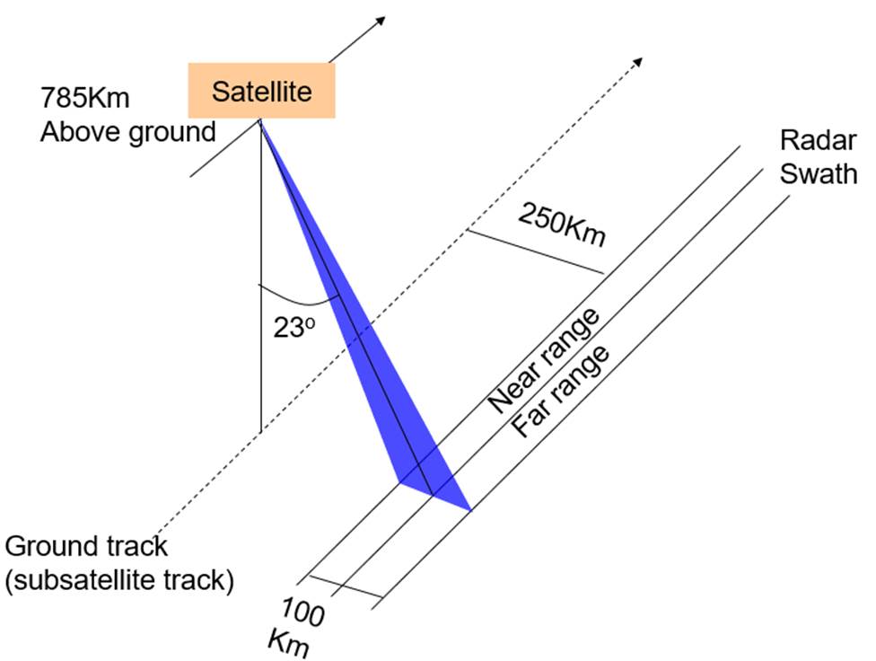
Figure 1. The side-looking radar system in ERS satellites.
Figure 2 shows three different angles in an SLR system. The look angle is measured from the nadir, and the depression angle is measured from the tangent of an ellipsoid. Incident angle indicates the angle between the incident beam and the normal to the ellipsoid. Local incident angle is different from the incident angle. Local incident angle is the angle between the incident beam and the normal to the ground surface.
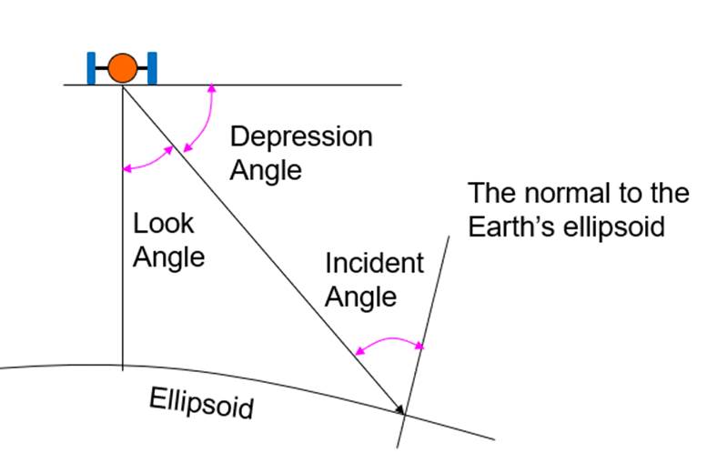
Figure 2. Three angles in SLR.
Determining Pixel Location
Unlike the passive sensor system of which pixel locations are determined by lens characteristics, pixel location in an SLR system is determined by slant range (SR), flying height (H), and ground range (GR), as shown in Figure 3.
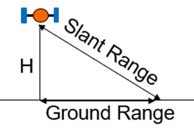
Figure 3. Slant range and ground range
Slant range is the distance between a radar transmitter and a ground object. Slant range is measured with the travel time of signal echoes. The equation for slant range calculation is [C x T / 2] where C is the velocity of light (3E+8 m/s). T is the travel time of a signal. In the equation, division by two is needed because T is a round-trip time. Ground range is calculated with the Pythagoras theorem, such that GR = (SR2 – H2)1/2. Figure 4 shows a slant range image and its ground range image. The slant range image shows compression along the look direction, i.e. right-hand side, during the ascending orbit.
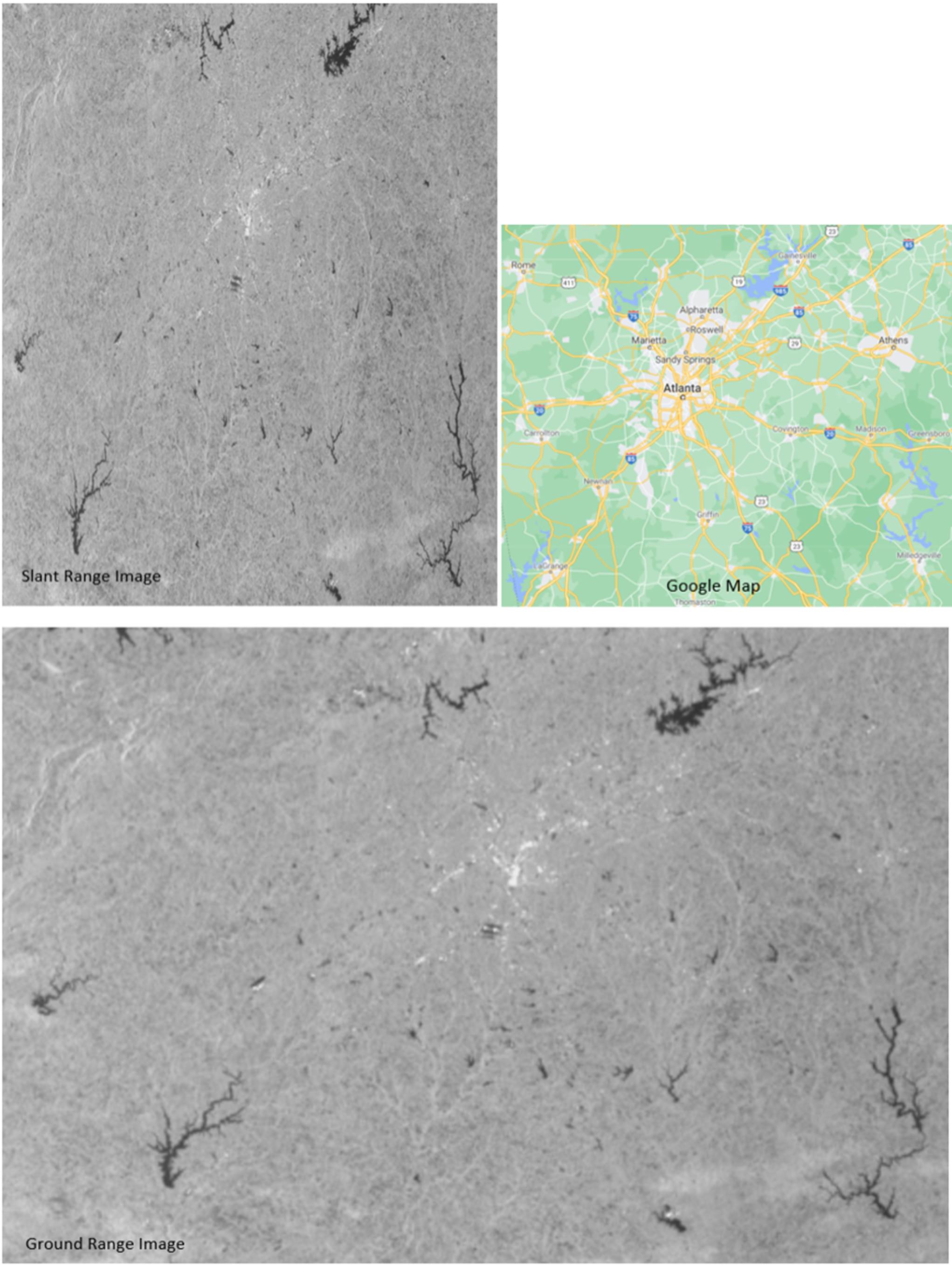
Figure 4. Slant image (top) vs. ground image (bottom). Atlanta and vicinity. September 11, 2020. Data source: Sentinel-1 C-Band data. Satellite flight direction: top. Look direction: right. Acquisition start time in UTC: 23:38:32.673120.
Relief and SLR Image
Because pixel locations are determined by the slant range, relief representation is quite different from that of air photos. In radar images, layover, foreshortening and radar shadows may occur as shown in Figure 5.
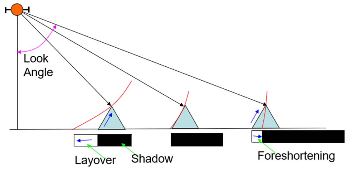
Figure 5. Layover, radar shadow, and foreshortening.
In the case of a very steep slope, if a target in a valley has a larger slant range than a neighboring mountain top along the look direction, then the foreslope is "reversed" in the slant range image. This phenomenon is called layover: the ordering of surface elements on the radar image is the reverse of the ordering on the ground. Generally, these layover zones, facing radar illumination, appear as bright features on the image due to the low incidence angle. Foreshortening is the phenomenon that foreslopes are compressed. Foreshortening happens frequently in high mountainous areas. The backslope of a high mountain is not reached by any radar beams, making radar shadow in the image. Radar shadow becomes longer as the look angle increases.
Pixel Resolution of a Radar Image
The pixel size in a radar image is determined by range resolution and azimuth resolution. Range resolution is the resolution along the beam range direction. Azimuth resolution is the resolution across the beam width. Figure 6 shows equations for calculating the azimuth and range resolutions. Range resolution is calculated as CT / (2 ž cos(θ)), where C is the speed of light (3E+8 m/s), T is pulse duration (i.e. How long each pulse lasts), and θ is depression angle. As indicated in the equation, range resolution gets bigger (i.e. longer pixel size) as pulse duration increases. Azimuth resolution is calculated as a slant range multiplied by antenna beam width. As beam width increases, azimuth resolution gets bigger (i.e. larger pixel size).
In radar systems, beam width is inversely proportional to the antenna length. Specifically, BeamWidth = WaveLength / AntennaLength. Therefore, azimuth resolution = SlantRange x Wavelength / AntennaLength. This indicates that azimuth resolution is inversely proportional to the antenna length.
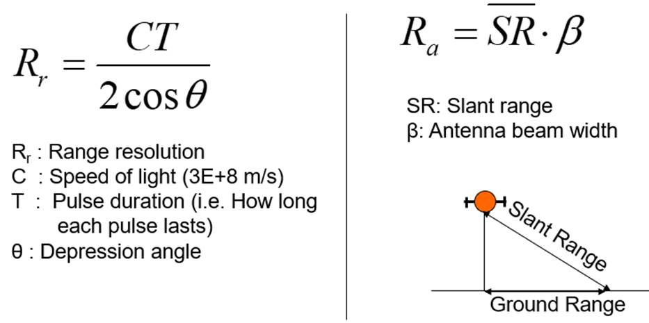
Figure 6. Equations for calculating range resolution and azimuth resolution
Suppose that an SLR system transmits pulses over a duration of 0.2 μsec. The range resolution at a depression angle of 45o will be 300000000 x 0.0000002 / (2 x cos(45o)), which is 42.4m. Also, suppose that an SLR system has a 2.0-mrad antenna beam width. The azimuth resolution at the slant range of 12 km will be 12000 x 0.002, which is 24 meters.
Synthetic Aperture Radar (SAR)
As indicated in the azimuth resolution equation (azimuthResolution = groundResolution x wavelength / antennaLength), one way of obtaining high-resolution data is to make the physical antenna length longer, or the wavelength shorter. We call these systems brute force, real aperture, or noncoherent radars.
Another way is to create a long antenna mathematically from a short physical antenna (i.e. creating a synthesized antenna). We call this a Synthetic Aperture Radar (SAR) system. SAR is used by most radar imaging systems nowadays.
Polarization
Another important characteristic of radar imaging is the use of the polarization technique. The signals sent or received can be polarized because objects may reflect signals directionally. Minerals are especially prone to polarize microwave wavelengths. Images that record polarization may contain more information. Horizontal and vertical polarization methods are used in radar imaging. Considering sending and receiving signals, there are four possible combinations of polarization.
1. Horizontal sending and horizontal receiving (HH polarization)
2. Horizontal sending and vertical receiving (HV polarization)
3. Vertical sending and horizontal receiving (VH polarization), and
4. Vertical sending and vertical receiving (HH polarization)
HH and VV polarizations are called Like-Polarization. HV and VH polarizations are called Cross-Polarization. If a system has HH, VV, HV, and VH, it is called Quadrature Polarization.
Radar Image Interpretation
Foreshortening, Layover, and Radar Shadow
Radar images show foreshortening or layover if an object’s relief is high. Figure 7 shows foreshortenings in the Himalayan Mountains. Radar shadows also appear in the high mountain areas.
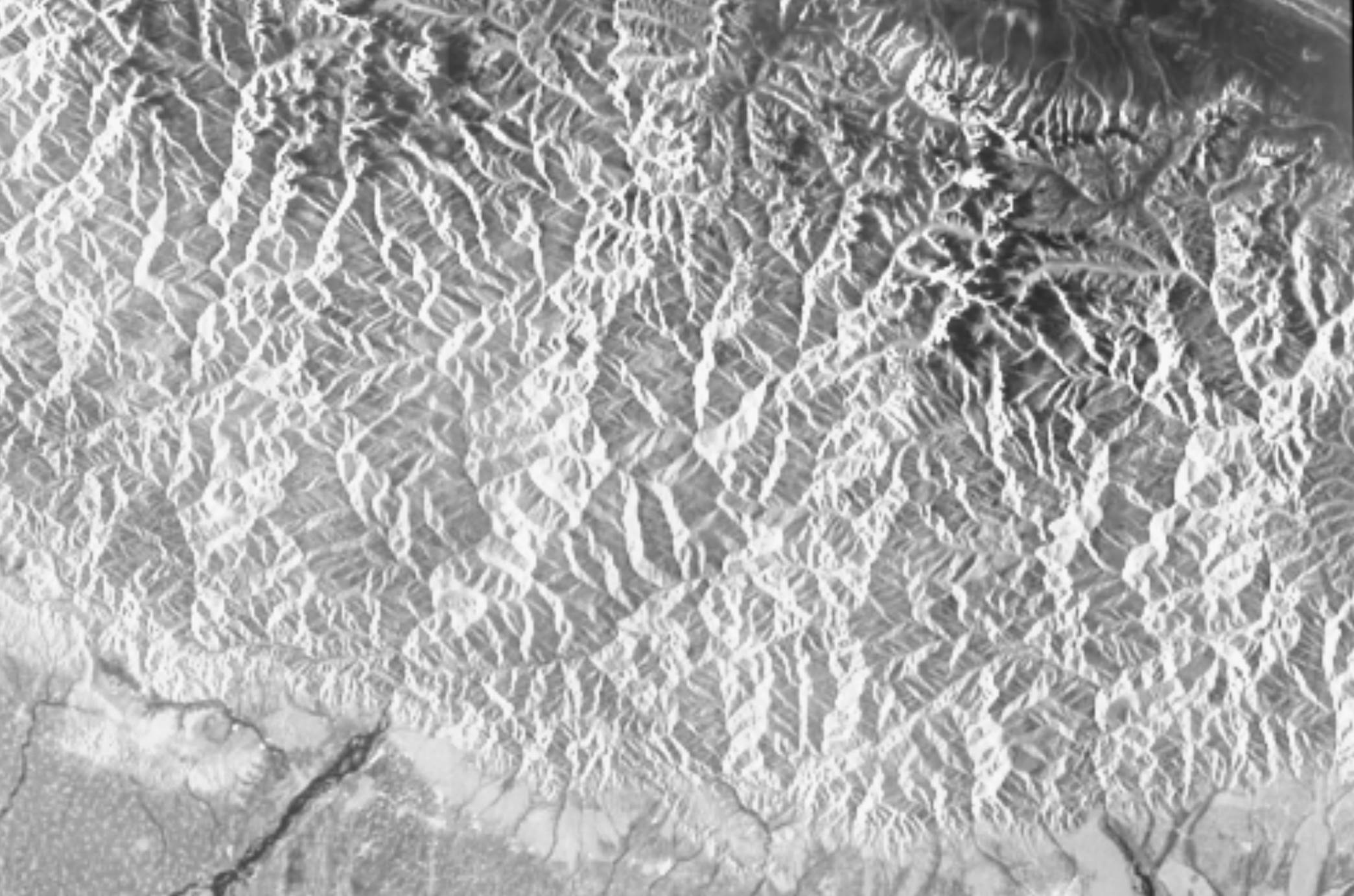
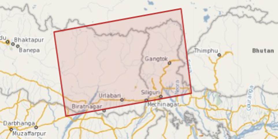
Figure 7. Sentinel-1A ground range image. Himalaya Mountains area. 2020-08-23.
Speckle
Another important feature appearing in radar images is speckles. During radar imaging, each cell associated with a target contains several scattering centers whose elementary returns, by positive or negative interference, originate light or dark image brightness. Speckle, therefore, is a system phenomenon and is not the result of spatial variation of average reflectivity of the radar illuminated surface. To remove speckles, two approaches have been used. One is multi-look processing which takes an average of multiple looks. The other is filtering techniques that apply various moving window filters. You need to be careful when using these approaches because they inevitably reduce spatial resolution. Shown Figure 8 is an example of speckles.
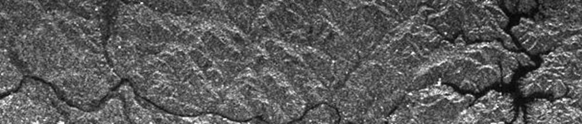
Figure 8. Speckles in a radar image.
Brightness Level
Another important thing to remember in interpreting radar images is that the pixel brightness level is not related to solar illumination. The brightness level in radar images is related to the relative strength of the microwave energy backscattered by the landscape elements. Shadows in radar images are related to the oblique incidence angle of microwave radiation emitted by the radar system and not to the geometry of solar illumination.
Brightness level is affected by wavelength, polarization, look angle, object roughness, shape geometry, and dielectric properties. Figure 9 shows how different wavelengths backscatter against some Earth objects. It shows that longer wavelengths backscatter more in-depth. At short wavelengths like the X band, the surface reflectance characteristics determine the brightness level of the radar image. However, as wavelengths increase, the variation of brightness level reflects not only the surface objects but also subsurface objects. It should also be noted that penetration depth is also related to the moisture of the target. Specifically, microwaves do not penetrate water more than a few millimeters.
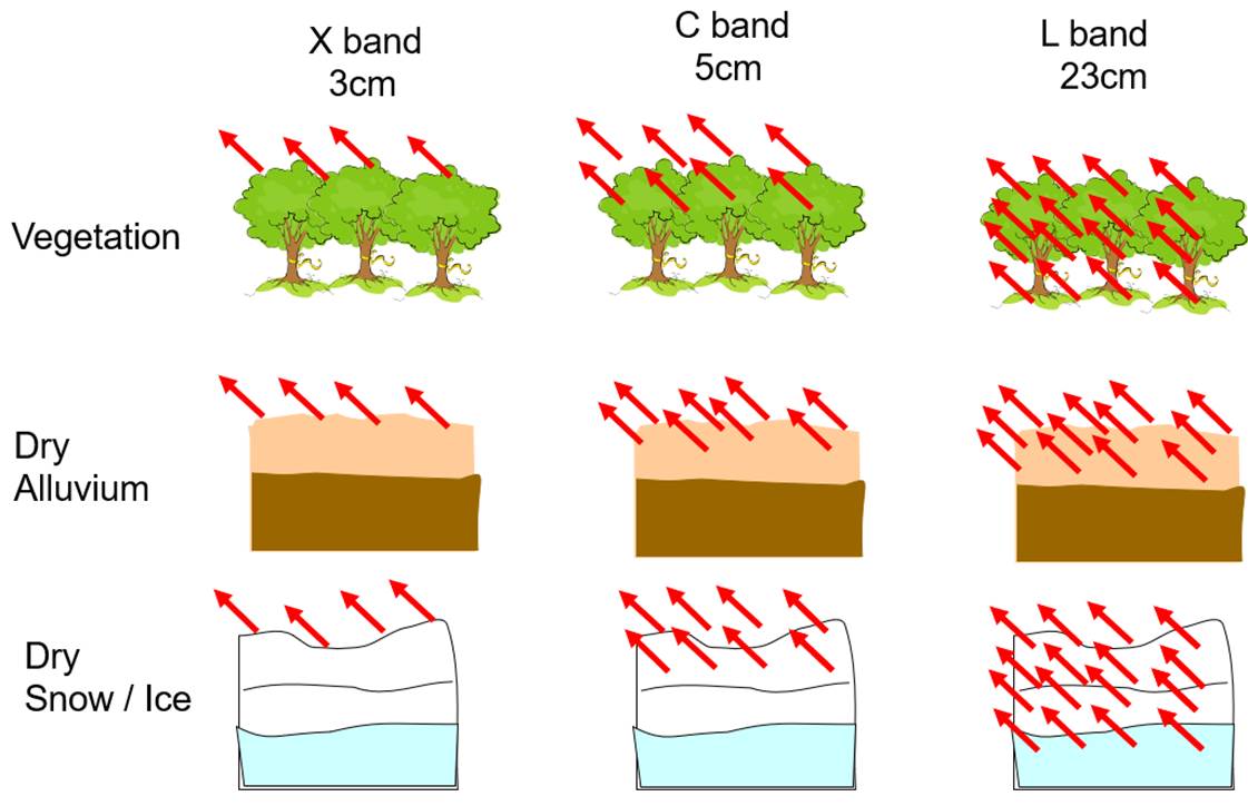
Figure 9. Backscattering of different wavelengths against some Earth objects.
Roughness and Backscattering
Surface roughness is a very important factor affecting brightness levels. In general, Urban areas backscatter strongly. Forests scatter intermediately, and calm water weakly. The Amazon image in Figure 10 shows grayish intermediate backscatters. The Beijing image at the bottom shows strong backscatters in urban areas.
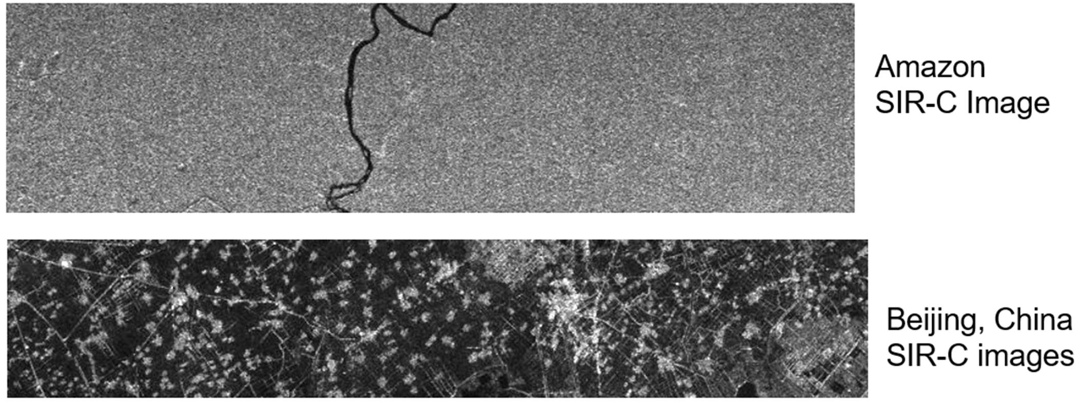
Figure 10. Roughness and backscattering
Dielectric Properties
Dielectric properties in objects also affect backscattering. In the microwave region of the spectrum, most natural materials have a dielectric constant in the range of 3 to 8 when dry. Water has a dielectric constant of 80. Metal objects (ex. bridges, silos, railroad tracks, and poles) have a high dielectric constant. The dielectric constant is strongly related to moisture levels in objects. Tone, therefore, becomes brighter as the dielectric value becomes higher.
Radar Image Processing
Radar image processing may require multiple steps depending on pre-processing levels and applications. One typical goal of SAR image processing is to create a terrain-corrected and georeferenced (projected) radar backscatter image.
Table 1 shows SAR image processing levels.
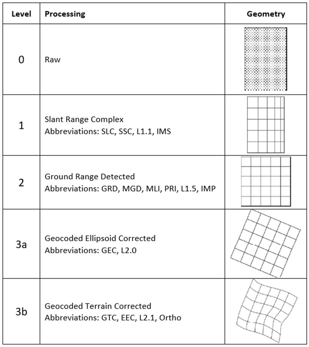
Table 1. SAR image processing levels. (Braun, 2019)
In this section, a Sentinel-1 SLC image (S1A_IW_SLC__1SDV_20191222T233825_20191222T233853_030468_037CEF_FA82.zip) was used with the SNAP software package (http://step.esa.int/main/download/snap-download/) to show some processing steps and results. Figure 11 shows the bands that come with the SLC image and the Intensity_IW1_VV image.
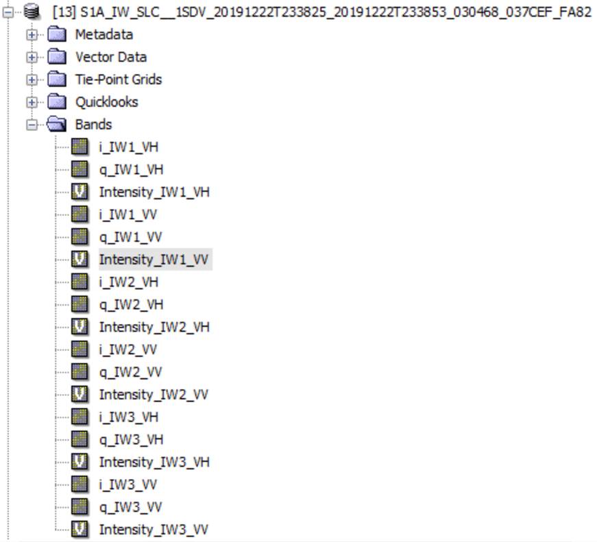
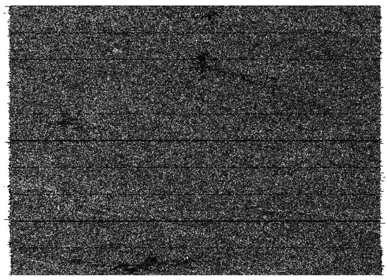
Figure 11. The bands that come with a Sentinel-1 SLC image and the Intensity_IW1_VV image.
Processing the Level 1 SLC image typically requires the following steps to create a terrain-corrected, backscatter coefficient image. The SNAP toolkit (http://step.esa.int/main/doc/tutorials/) was used to process the steps.
1. Apply Orbit File
The orbit information provided in the metadata of a SAR product is generally not accurate and can be refined with the precise orbit files which are available days-to-weeks after the generation of the product.
2. Radiometric Calibration
SAR radiometric calibration is to change pixel values so that they are directly related to the radar backscatter of the scene. Calibrated SAR images are essential to the quantitative use of SAR data. Level 1 images, often, do not include radiometric corrections, and significant radiometric bias remains. The radiometric correction is also necessary for the comparison of SAR images acquired with different sensors, acquired from the same sensor but at different times, in different modes, or processed by different processors. Radiometric correction creates a Sigma0 (“Sigma naught”) image for each band. Figure 12 shows a radiometric calibration result.
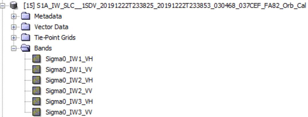
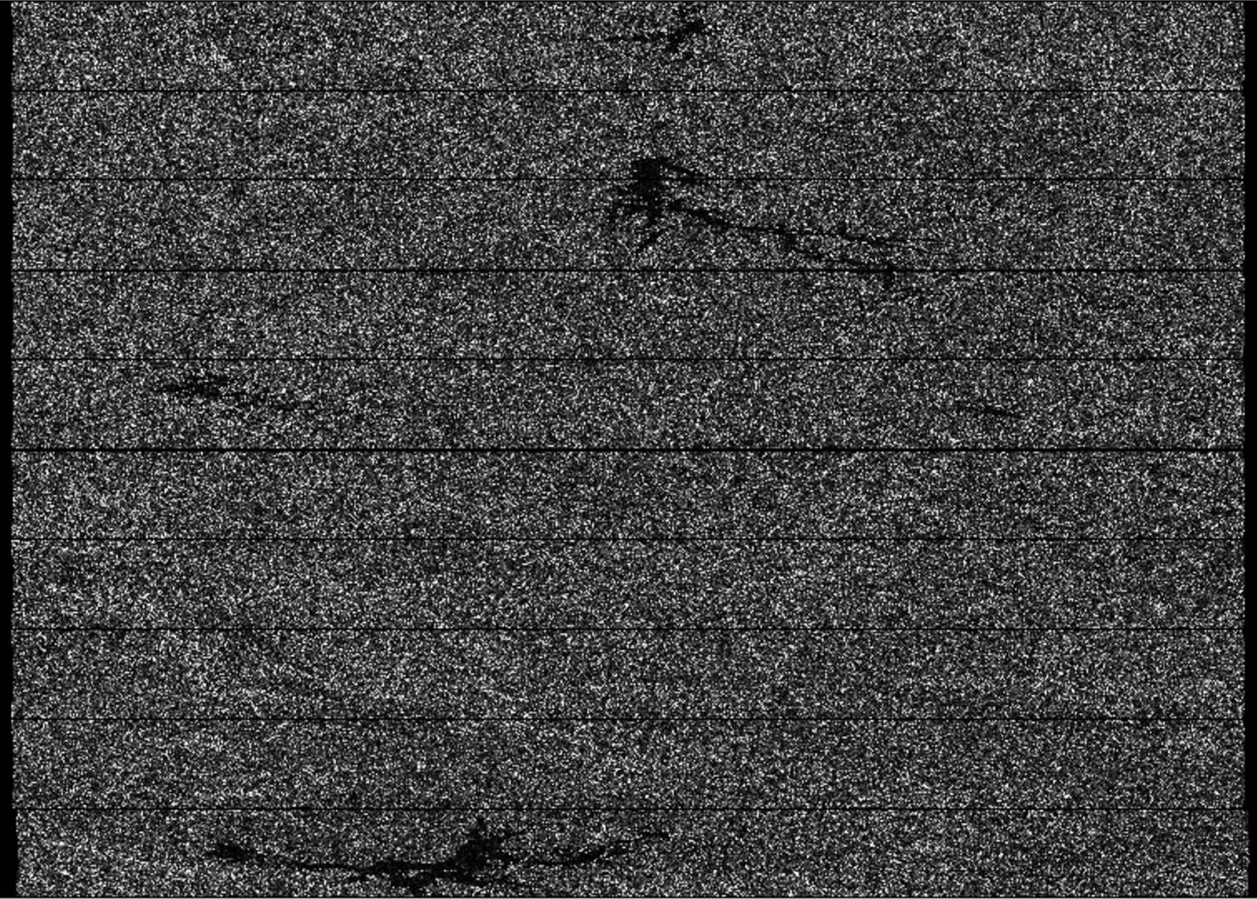
Figure 12. Result of radiometric calibration. Image band: Sigma0_IW1_VH.
3. TOPS Deburst
Terrain Observation with Progressive Scans (TOPS) data is acquired in bursts. Each burst is separated by demarcation
Zones (i.e. horizontal dark lines) as shown in Figure 12. Any data within the demarcation zones can be considered invalid. TOPS Deburst removes the demarcation zones and merges multiple bursts as shown in Figure 13.
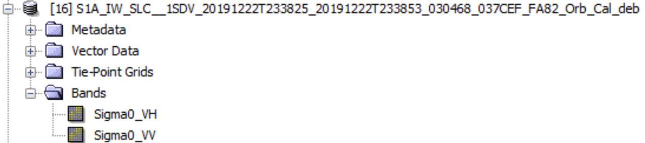
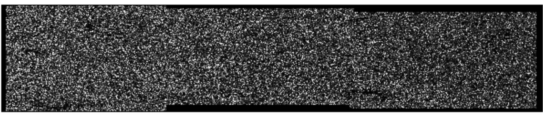
Figure 13. Result of deburst that shows no demarcation zones. Image band: Sigma0_VH.
4. Multilooking
Generally, a SAR original image appears speckled with inherent speckle noise. To reduce this inherent speckled appearance, several images are incoherently combined as if they corresponded to different looks of the same scene. This processing is generally known as multilook processing. The multilooked image improves the image interpretability. Also, multilook processing can be used to produce an application product with a nominal image pixel size. Figure 14 shows the result of applying the multilook process.
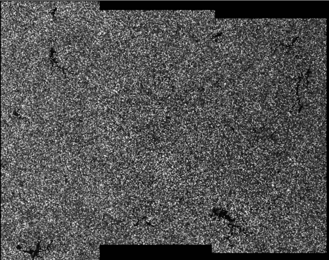
Figure 14. Result of multilook processing.
5. Range-Doppler Terrain Correction
Terrain corrections compensate for the distance distortions caused by topographic variations in the real world. During the range-Doppler terrain correction, orthorectification with a DEM, radiometric normalization, and map projection processes are typically performed. Figure 15 shows the result of terrain correction. The output coordinate system is UTM Zone 16 N with the WGS84 datum. Before the terrain correction, the north direction pointed the bottom, and the image was flipped vertically. After geocoded terrain correction, the image shows a correct orientation so that the images can be aligned with other layers in a GIS system or Google Earth Pro.
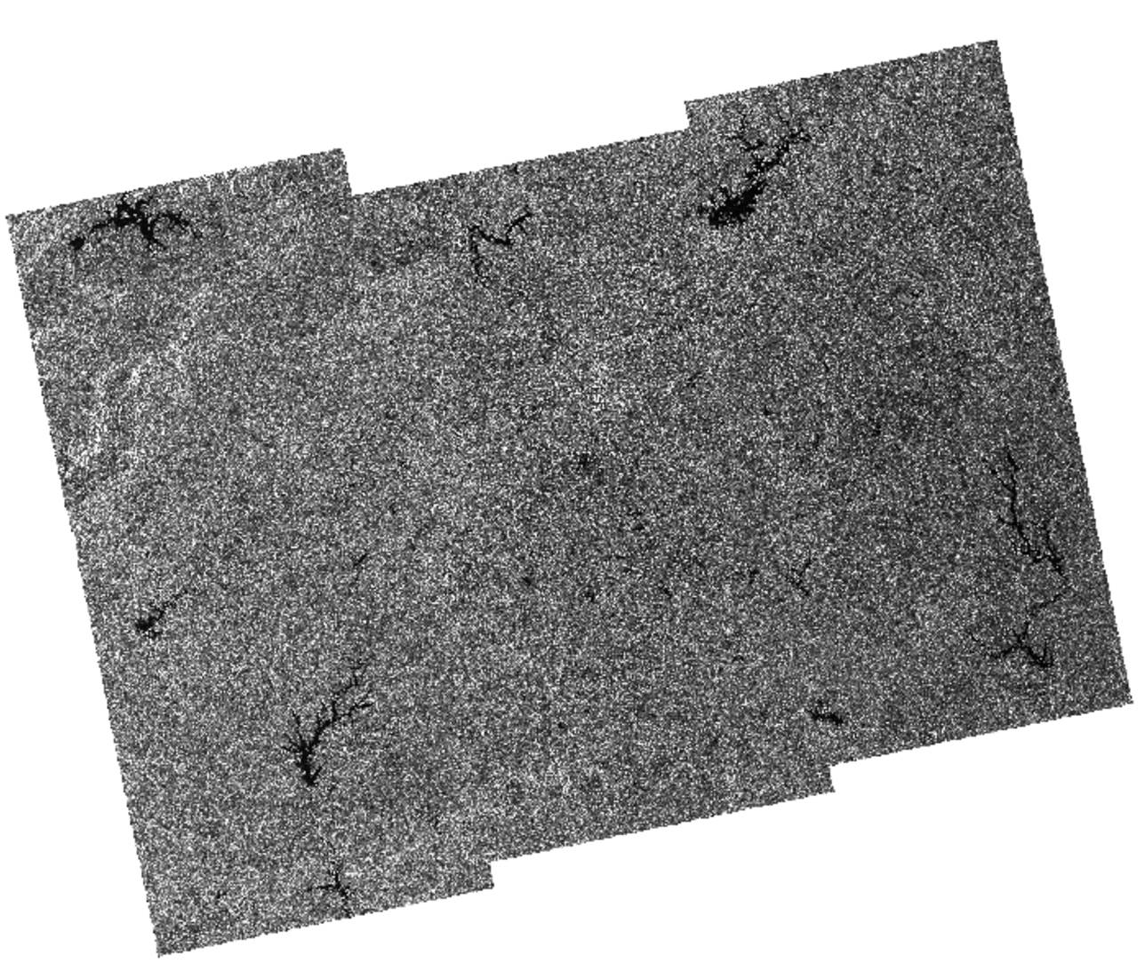
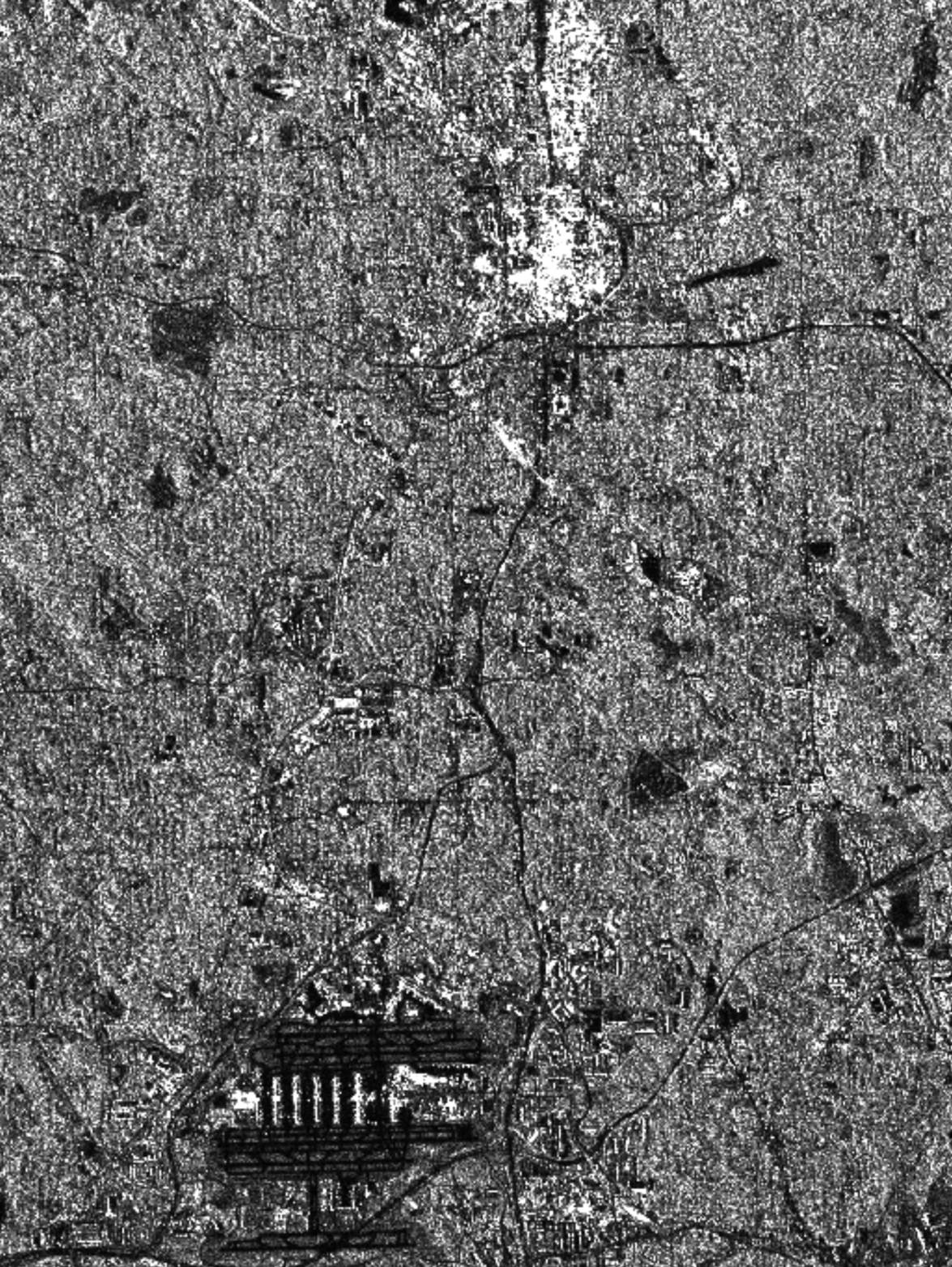
Figure 15. Range-Doppler terrain correction image. Top: Entire scene. Bottom: An enlarged image showing the Atlanta downtown and the Atlanta Hartsfield International Airport.
References
Andreas Braun, 2019. Radar satellite imagery for humanitarian response: Bridging the gap between technology and application. Dissertation. Eberhard Karls Universität Tübingen. https://publikationen.uni-tuebingen.de/xmlui/handle/10900/91317