Image Classification
Image classification is the processes of grouping image pixels into
classes of similar types. A typical example of using image classification is
the land cover identification from remotely sensed images. This chapter focuses
on land cover classification techniques.
Land Cover Classification Scheme
There are many categories or classes that we can derive from an image.
There are some image classification schemes frequently used. The most
popular landuse/landcover classification scheme
is the Anderson’s classification scheme developed by the U.S. Geological Survey
in 1976. It uses a hierarchical structure in multiple levels. Level I has nine
categories as shown in Figure 1. Level II has more detailed categories, and,
with further details, the Anderson’s classification
scheme goes down up to Level IV. Figure I shows that
Forested Land, for example, is further divided into three classes in Level II.
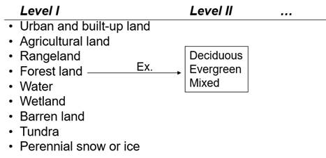
Figure 1. USGS land cover classification scheme by Anderson, et al.
(1976)
Patterns used for Image Classification
Three patterns in an image are frequently used for image classification –
spectral pattern, temporal pattern, and spatial pattern. With a
multispectral dataset, we can classify pixels by examining the spectral profile
in each pixel. With a multitemporal dataset, temporal patterns can also be
analyzed to determine the category of a pixel. In this case, plant phenology is
frequently used. Plant phenology is the study of the annual cycles of plants
and how they respond to seasonal changes in their environment. For example,
there will be little greenness on deciduous trees in winter, but high greenness
levels during summer. Spatial patterns are also used to classify an image.
Particularly, texture, size, shape, and directionality are frequently used.
Figure 2 shows a Landsat 8 OLI image and a spectral pattern on a wooded land.
Band 5 (i.e. the near infrared band) shows very high reflectance compared with
other bands.
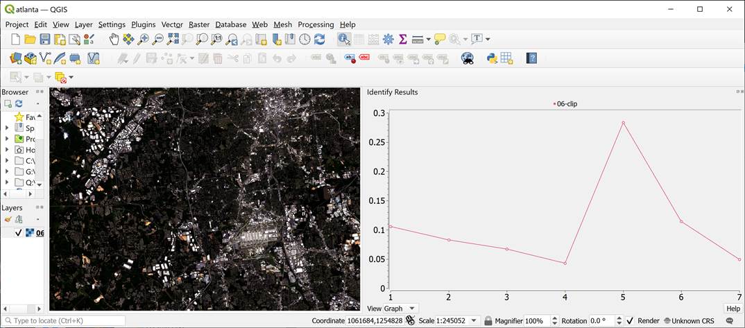
Figure 2. A spectral pattern of a wooded land in Atlanta, GA. Landsat 8
OLI ARD image. (May 6, 2020)
Classification Approaches
There are four classification approaches frequently used as shown below.
· Pixel-based image classification
o Unsupervised
o Supervised
· Object-based image classification
o Unsupervised
o Supervised
The pixel-based approach clusters pixels using their spectral or temporal
profile. The object-based image analysis (OBIA) creates polygonal objects by
clustering neighboring pixels by looking at their statistical properties such
as texture, size, shape, or directionality. Both approaches can be combined
with either unsupervised or supervised approaches.
As shown in Figure 3, unsupervised classification classifies pixels into
groups with iterative statistical algorithms, and then, the meaning of each
group is later identified in relation to ground features. Supervised
classification uses a different approach. First, statistical signatures are
derived from a training dataset. And then, each pixel is compared with
statistical signatures to find out the best-fit category. Eventually, the
category of the best-fit signatures is assigned to the pixel.
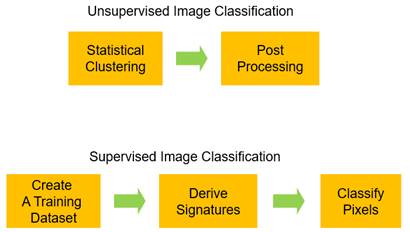
Figure 3. Unsupervised vs. supervised image classification procedures.
Creating a Training Dataset
A training dataset needs to be created carefully. A training dataset is
composed of multiple training samples. Training samples must clearly represent
the land cover classes of interest. Each training sample site needs to be
homogeneous.
Enough pixels need to be collected for each class. The Minimum in
practice is [10 x # of bands]. For example, if seven bands from the OLI sensor
are used for image classification, at least 70 pixels needs to be collected for
each class.
Training samples can be collected from a field survey (i.e. in
situ collection) or from a screen digitizing.
Each polygonal area delineated by screen digitizing is called AOI (area of
interest) or ROI (region of interest). Figure 4 shows training samples in
different colors. The training dataset was used for the supervised
classifications described in this chapter.
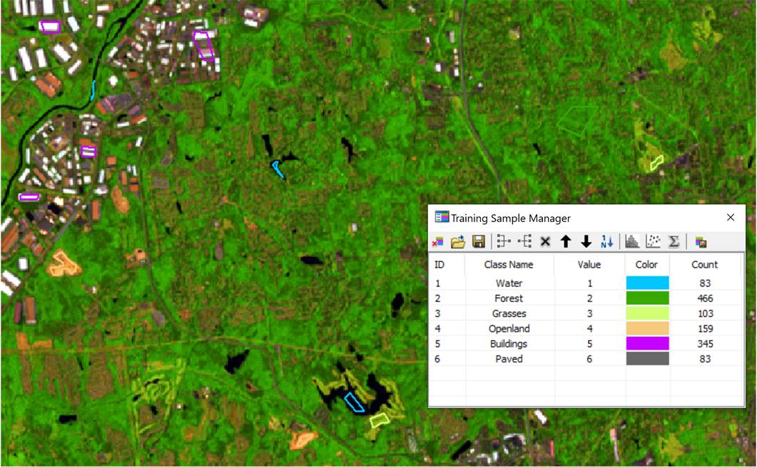
Figure 4. Training samples in a training dataset.
Classification Tools
Many software packages provide image classification tools. With the
development of machine learning algorithms, various image classification
algorithms have been developed too. The following lists popular software
packages that provides advanced image
classification methods:
· Opensource
o SAGA. http://www.saga-gis.org/en/index.html
o The Caret package for R. http://topepo.github.io/caret/index.html
o OpenCV and TensorFlow in
Python. https://www.python.org/
o WEKA for ImageJ. https://imagej.net/Trainable_Segmentation
· Commercial
o ERDAS Imagine. https://www.hexagongeospatial.com/products/power-portfolio/erdas-imagine
o ENVI. https://www.l3harrisgeospatial.com/Software-Technology/ENVI
The examples presented in this chapter were developed with the SAGA
(System for Automated Geoscientific Analysis) Version 7.7.0 that provides the
following image classification tools:
· K-Means Clustering for Grids
· ISODATA Clustering
· Decision Tree
· Supervised Classification for Grids
o Binary Encoding
o Parallelepiped
o Minimum Distance
o Mahalanobis Distance
o Maximum Likelihood
o Spectral Angle Mapping
o Winner Takes All
· Supervised Classification for Shapes
· Supervised Classification for Tables
· Seeded Region Growing
· Superpixel Segmentation
· Watershed Segmentation
· Object Based Image Segmentation
· SVM (Support Vector Machine) Classification
· Artificial Neural Network Classification (OpenCV)
· Boosting Classification (OpenCV)
· Decision Tree Classification (OpenCV)
· K-Nearest Neighbours Classification
(OpenCV)
· Normal Bayes Classification (OpenCV)
· Random Forest Classification (OpenCV)
· Random Forest Table Classification (ViGrA)
The K-means clustering is a pixel-based unsupervised classification
method. It starts by partitioning the input pixels into k initial clusters,
either at random or using some heuristic data. It then calculates the mean of each cluster. It constructs a new partition by
associating each pixel with the closest mean.
Then the mean values are recalculated for the new clusters, and the algorithm
is repeated by applying these two steps until convergence, which is obtained
when the pixels no longer switch clusters (or alternatively, mean values are no
longer changed). Figure 5 shows the output of K-means clustering with 4
categories.
Once pixels are grouped into clusters, the clusters need to be named to
reflect ground features. In this procedure, multiple clusters can be combined
to one. For example, the clusters in gray, red, and sand colors in Figure 5 may
be combined to the built-up class
that includes roads, buildings, and pavements.
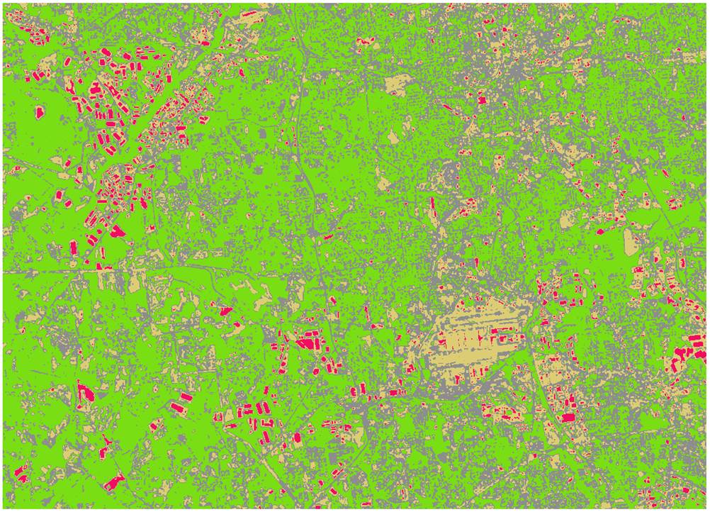
Figure 5. K-means clustering with 4 classes.
The ISODATA clustering is another pixel-based unsupervised classification
method. ISODATA stands for iterative self-organizing data analysis technique. The ISODATA clustering algorithm has some further
refinements by splitting and merging of clusters. Clusters are merged if either
the number of pixels in a cluster is less than a certain threshold or if the
centers of two clusters are closer than a certain threshold. Clusters are split
into two different clusters if the cluster standard deviation exceeds a predefined value and
the number of pixels is twice the threshold for the minimum number of members.
Unlike the k-means algorithm, the ISODATA algorithm allows for a different
number of clusters in output. Figure 6 shows the result of ISODATA clustering.
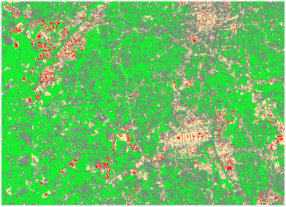
Figure 6. ISODATA clustering with 4 classes.
The minimum distance method is a supervised image classification
technique. In the minimum distance method, the distance between the mean of the signature dataset and the pixel value
is calculated band-by-band. Then, a total distance is calculated. This
total-distance calculation routine is repeated with all class signatures. The
class that shows the minimum total distance is assigned to the pixel. This
minimum distance method is very fast and simple in its concept. Figure 6 shows
the result of minimum distance classification.
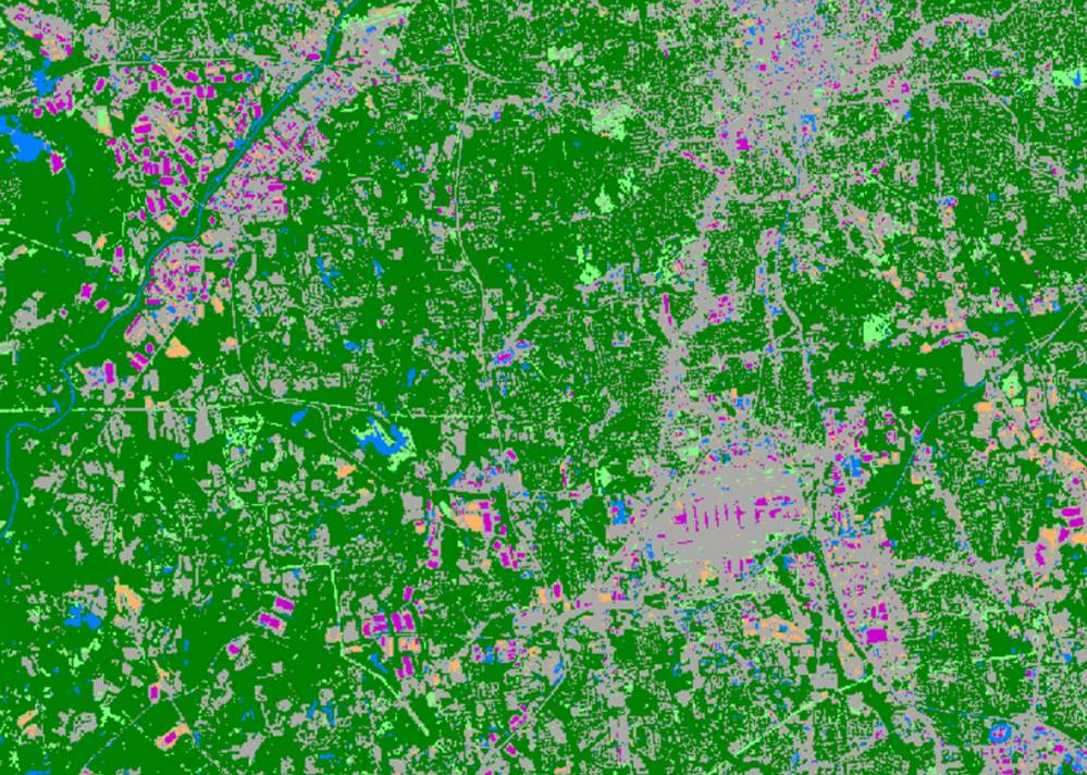
Figure 6. Minimum distance classifier
The maximum likelihood classifier (MLC) considers statistical probability
of the class signatures when deciding the class that a pixel belongs to. The
maximum likelihood method should be used Carefully. First, sufficient training
samples should be used with this method. Second, if there are very high
correlations among bands or if the classes in the training dataset are very
homogeneous, results are unstable. In such cases, users may consider reducing
the number of bands using the principal component transformation. Third, when
the distribution of training samples does not follow the normal distribution,
the maximum likelihood method will not perform well. Figure 7 shows the result
of MLC classification. Paved land covers like roads and parking lots are classified to Buildings. Also, residential areas are classified to
Grasses.
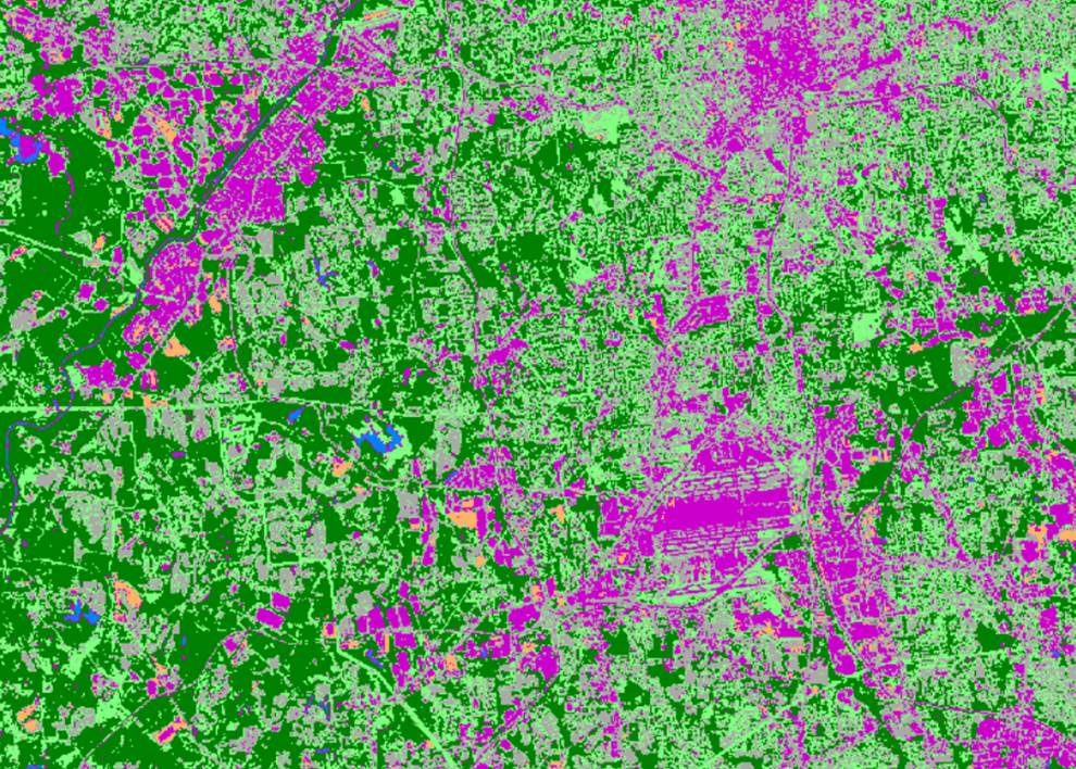
Figure 7. Maximum likelihood classifier.
The decision tree method is a supervised classification technique that
uses a training dataset. A decision tree is a connected graph with a root node
and one or more leaf nodes in a tree shape. A decision tree can be built
manually, or with machine learning from a training dataset. Once a decision
tree is created, pixels can be classified using it. Figure 8 shows the result
of applying decision tree classification method. The figure shows that multiple
roads are confused with grasses. Also, pavements
are not well separated from buildings.
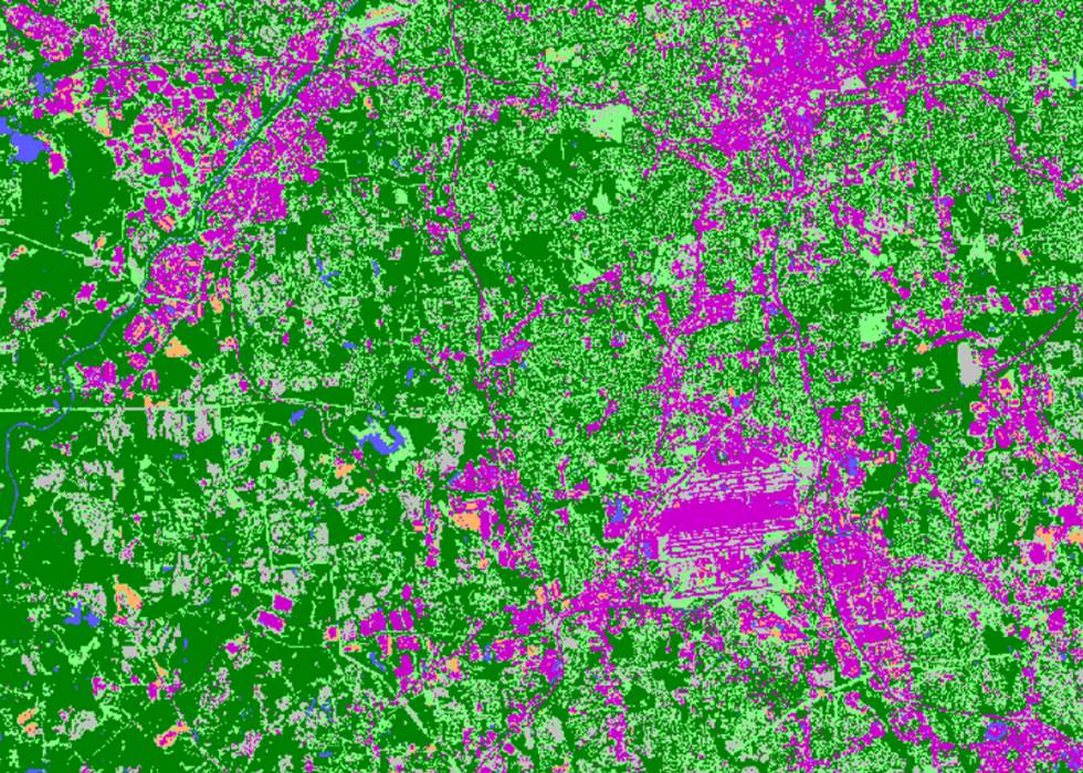
Figure 8. Decision tree classifier.
The random forest method is a supervised classification technique and
uses a machine learning algorithm. As a frequently used method, the random
forest classifier uses multiple decision trees, making a forest. Figure 9 shows
the result of applying the random forest classifier with the following
parameters, and the result is similar to the
decision tree classifier.
· Maximum tree depth: 10
· Minimum sample count: 2
· Maximum categories: 6
· Use 1SE rule: No
· Truncate pruned trees: no
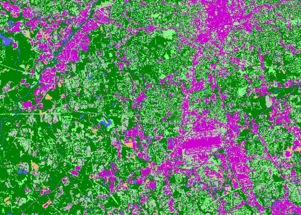
Figure 9. Random forest classifier.
The neural network classifier is a supervised classification method that
uses machine learning algorithms. Figure 10 shows an output using the neural
network classifier with the following parameters:
· Number of layers: 3
· Number of neurons: 6
· Maximum number of iterations: 300
· Error change (epsilon): 0.0000001192
· Activation function: Sigmoid (alpha = 1, beta = 1)
· Training method: back propagation (weight gradient term =
0.1, moment term = 0.1)
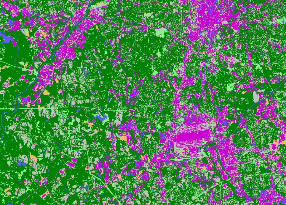
Figure 10. Neural network classifier.
Object-Based Image
Analysis (OBIA)
OBIA starts with segmenting an image into multiple polygons, i.e.
objects, by grouping pixels using such information as
shape, texture, spectral properties, and geographic proximity. The polygons are
further merged into classes using supervised or unsupervised clustering
methods. Figure 11 shows polygon objects, and Figure 12 shows the result of
unsupervised OBIA classification with the following parameters:
· Band width for seed point generation: 2
· Neighborhood determination: 4 direction (Neumann
neighborhood)
· Distance determination: Feature space and position
o Variance in feature space: 1
o Variance in position space: 1
o Similarity threshold: 0
· Generalization: No generalization
· Number of unsupervised classification classes: 6
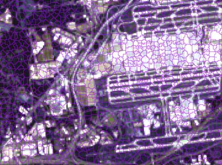
Figure 11. Polygon objects
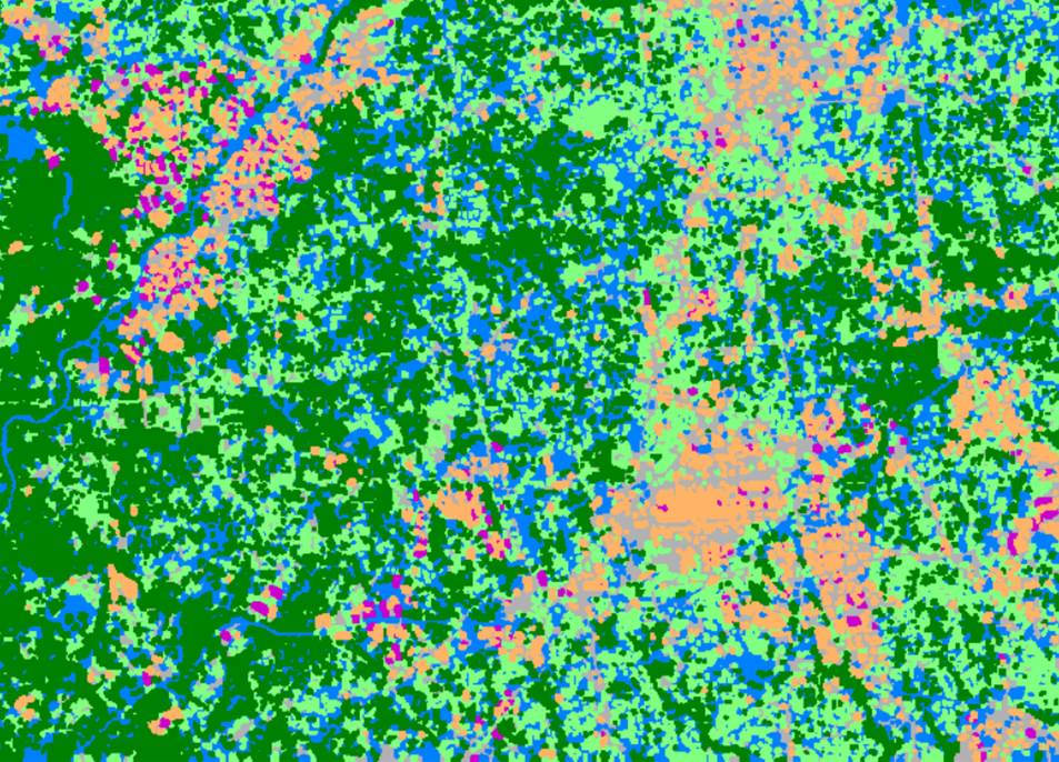
Figure 12. OBIA classification, unsupervised.
Classification
Accuracy Assessment
Once an image is classified, the accuracy of the classification should be
assessed. An error matrix is frequently used for checking errors. The error
matrix is also known as a “contingency table,” or “confusion matrix.” Enough
cases should be sampled to test classification errors. In general, 50 cases per
class are recommended. If the study area is larger than 1 million acres, or if
there are more than 12 categories, 75-100 cases per category are recommended.
When selecting sample cases, random or stratified random sampling would bring
less biased assessment. Testing results are organized as shown in Table 1.
Columns represent classification results, and rows represent reference
data. The value of 64 in the
table, for example, means that 64 Water pixels in reality
were classified to Conifer, which
means an error.
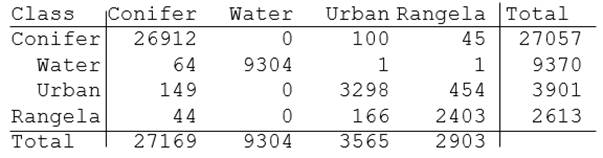
Table 1. An error matrix (example)
When assessing classification accuracies, we need to check them from two
standpoints – producer’s and user’s. From a
producer’s standpoint, what is important is how well the original features are
represented in the classification output. This is what we call producer’s
accuracy. Producer’s accuracy is calculated in association with reference data.
However, in a user’s perspective, what is important is how
much the classification results are accurate. This is, what we call, user’s
accuracy. The user’s accuracy is calculated in association with classification
results. Table 2 shows how to calculate producer’s accuracy, user’s accuracy,
and overall accuracy. In the table, the capital letters A – P indicate numbers.
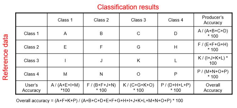
Table 2. Accuracy calculation
Table 3 shows an example of producer’s accuracy and user’s accuracy. For
example, 92.51% of urban areas are represented in the classification result,
and only 84.54% of urban pixels are truly urban. The overall accuracy is 97.6%.
Even if the overall accuracy is a good indicator of an image
classification accuracy, the overall accuracy may change if another sample
dataset is used.
The KHAT statistic takes potential sampling errors into account, so that
KHAT is more robust than the overall accuracy. KHAT and the overall accuracy
range from 0.0 to 1.0. Conventionally, the KHAT values less than 0.4 are
considered a very poor classification.
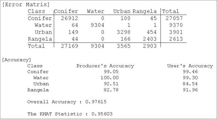
Table 3. An accuracy test result (example)
James R. Anderson, Ernest E. Hardy, John T. Roach, and Richard E. Witmer,
1976. A land use and land cover classification system for use with remote
sensor data. Professional Paper 964 (A revision of the land use classification
system in Circular 671). https://doi.org/10.3133/pp964.